Machine learning

Week 4: optimization and model fitting

Joshua Loftus

LSE

Week 4: optimization and model fitting

Part 1: fitting logistic regression

Part 2: empirical risk minimization and gradient descent

Part 3: stochastic gradient descent

Part 4: where the error comes from, this time

Part 5: stopping

Where week 3 left the fitting

Week 2, least squares: \(\hat\beta\) solves the normal equations \(\mathbf X^\top(\mathbf y - \mathbf X\hat\beta) = \mathbf 0\), and there is a formula, \(\hat\beta = (\mathbf X^\top\mathbf X)^{-1}\mathbf X^\top\mathbf y\).

Week 3: logistic regression is fitted by maximum likelihood. How glm does it: this week

Write down the normal equations from memory. Then guess: what plays their role for logistic regression, where the fitted values are probabilities \(\hat p_i\) instead of \(\mathbf x_i^\top\hat\beta\)?

Fitting logistic regression

How do we estimate \(\beta\)? Maximum likelihood:

\[ \text{maximize } L(\beta ; \mathbf y | \mathbf X) = \prod_{i=1}^n L(\beta ; y_i | \mathbf x_i) \] (assuming the data is i.i.d.)

Next slide: a bit of mathematics

MLE

\[ L(\beta ; \mathbf y | \mathbf x) = \prod_{i=1}^n \left( \frac{1}{1+e^{-x_i \beta}} \right)^{y_i} \left(1- \frac{1}{1+e^{-x_i \beta}} \right)^{1-y_i} \]

\[ \ell(\beta ; \mathbf y | \mathbf x) = \sum_{i=1}^n y_i \log \left( \frac{1}{1+e^{-x_i \beta}} \right) + (1-y_i) \log \left(1- \frac{1}{1+e^{- x_i \beta}} \right) \]

MLE: the derivative

\[ \frac{\partial}{\partial \beta} \ell(\beta ; \mathbf y | \mathbf x) = \sum_{i=1}^n y_i \left( \frac{x_i e^{-x_i \beta}}{1+e^{-x_i \beta}} \right) + (1-y_i) \left(\frac{-x_i}{1+e^{- x_i \beta}} \right) \]

\[= \sum_{i=1}^n x_i \left[ y_i - \left(\frac{1}{1+e^{- x_i \beta}} \right) \right] = \color{#b73779}{\sum_{i=1}^n x_i [y_i - \hat p_i(\beta)]}\]

Set this equal to 0 and solve for \(\beta\). How: the rest of today

The score equations, read as orthogonality

Week 2, least squares: \(\mathbf X^\top(\mathbf y - \mathbf X\hat\beta) = \mathbf 0\). The residual is orthogonal to every column of \(\mathbf X\).

Logistic score equations. Stack the last slide’s rows: writing \(\mathbf p(\beta) = (\hat p_1(\beta), \ldots, \hat p_n(\beta))^\top\), the MLE \(\hat\beta\) solves \[ \mathbf X^\top\big(\mathbf y - \mathbf p(\hat\beta)\big) = \mathbf 0 \]

Same shape as least squares, with \(\mathbf X\hat\beta\) replaced by the fitted probabilities: the residual \(\mathbf y - \hat{\mathbf p}\) is orthogonal to every column of \(\mathbf X\)

No closed form, because \(\mathbf p(\beta)\) is not linear in \(\beta\)

Two things the score equations say

Row one is the intercept. \(\sum_i (y_i - \hat p_i) = 0\): the fitted probabilities average to the observed proportion of 1s on the training rows. An average identity for an unpenalized fit with an intercept, not calibration at each \(x\), and not a statement about new data.

The log-likelihood is concave. Differentiating once more, \[ \frac{\partial^2 \ell}{\partial\beta\,\partial\beta^\top} = -\sum_{i=1}^n \hat p_i(\beta)\,\big(1 - \hat p_i(\beta)\big)\, x_i x_i^\top \preceq 0, \] so any finite solution of the score equations is a global maximum, and the only one when \(\mathbf X\) has full column rank.

What concavity does not give: existence. Week 3’s separable case is the case with no finite solution.

Newton-Raphson

• Find the roots of a function
• Iteratively approximating the function by its tangent
• Root of the tangent line is used as starting point for next approximation
• See the animation on Wikipedia

Exercise: using result from previous slide, compute the second derivative of \(\ell\) and derive the expressions needed to apply Newton-Raphson

Logistic regression fitting: multivariate case

Newton-IRLS (equivalent) steps:

\[ \begin{eqnarray} \hat{\mathbf p}_t & = & g^{-1}(\mathbf X \hat \beta_t) & \ \text{ update probs.} \\ \mathbf W_t & = & \text{diag}[\hat{\mathbf p}_t (1 - \hat{\mathbf p}_t)] & \ \text{ update weights} \\ \hat{\mathbf{y}}_t & = & g(\hat{\mathbf p}_t) + \mathbf W_t^{-1}(\mathbf y - \hat{\mathbf p}_t) & \ \text{ update response} \end{eqnarray} \]

and then update parameter estimate (LS sub-problem) \[\hat{\beta}_{t+1} = \arg \min_{\beta} (\hat{\mathbf{y}}_t - \mathbf X \beta)^T \mathbf W_t (\hat{\mathbf{y}}_t - \mathbf X \beta)\]

Note: larger weights on observations with \(\hat p\) closer to 1/2, i.e. the most difficult to classify (look for variations of this theme) See Section 4.4.1 of ESL

Part 2: empirical risk minimization and gradient descent

ML tasks as optimization problems

For a given loss function \(\ell(y, f(x))\) and probability model \((X,Y) \sim P\), we want to find a function \(f\) to minimize risk:

\[ \text{minimize } R(f) = \mathbb E_P[\ell(Y, f(X))] \]

Math model \(\leftrightarrow\) Statistical model

Assume an i.i.d. sample from \(P\), focus on empirical risk minimization (ERM)

\[ \text{minimize } \hat R_n(f) = \frac{1}{n} \sum_{i=1}^n \ell(y_i, f(x_i)) \]

We also choose a function class \(\mathcal F\) (or parameter set), i.e. type of function \(f\), determining the domain of the optimization

Example: linear regression

Linear regression. Probability model: random errors \(\varepsilon \sim N(0, \sigma^2)\). Loss: squared, \(\ell(y, f(\mathbf x)) = (y - f(\mathbf x))^2\). Function class: \(\mathcal F = \{ f_\beta(\mathbf x) = \mathbf x^T \beta : \beta \in \mathbb R^{p+1} \}\). Algorithm: OLS, closed-form solution (memorized yet?)

\[\underset{\beta \in \mathbb R^{p+1}}{\text{minimize }} \frac{1}{n} \sum_{i=1}^n (y_i - \mathbf x_i^T \beta)^2\]

More examples: GLM

GLM. Probability model: family = binomial(), poisson(), etc. Loss: minus the log-likelihood of one row, so that \(\hat R_n(\beta) = -\ell(\beta)/n\). Function class: \(\{ g^{-1}(\mathbf x^T \beta) : \beta \in \mathbb R^{p+1} \}\), with a fixed link function \(g\). Algorithm: ERM (also MLE in this case) via iterative methods like Newton-Raphson or gradient descent

\[ \underset{\beta \in \mathbb R^{p+1}}{\text{minimize }} -\frac{1}{n} \sum_{i=1}^n \log L(\beta ; y_i | \mathbf x_i) \]

Optimization algorithms

Downside of Newton-Raphson: requires second derivatives, including inverting the \(p \times p\) Hessian matrix when optimizing over \(p > 1\) parameters

If \(p\) is large, second-order optimization methods like Newton’s are very costly

First order methods only require computing the \(p \times 1\) gradient vector

Recall that the gradient is a vector in the direction of steepest increase in the parameter space

Gradient (steepest) descent

i.e. skiing as fast as possible. Notation: the objective is the empirical risk \(\hat R_n(\beta)\), and \(t\) counts steps

1. Start at an initial point \(\beta_0\)

2. For step \(t = 1, \ldots\)

• Compute \(\mathbf d_t = \nabla \hat R_n(\beta_{t-1}) \color{#b73779}{\text{ (gradient)}}\)

• Update \(\beta_{t} = \beta_{t-1} - \gamma_t \mathbf d_t\)

3. Until some convergence criteria is satisfied

Where the step size \(\gamma_t > 0\) is made small enough to not “overshoot” and increase the loss, i.e. the loss only decreases

Which step size?

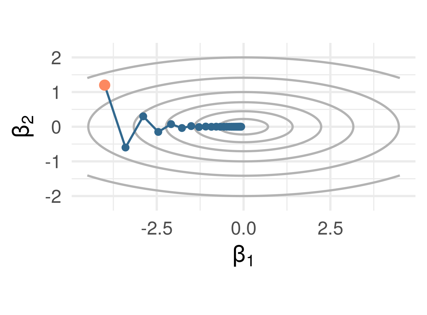
A valley, \(f(\beta) = \tfrac12(\beta_1^2 + 10\beta_2^2)\), ten times steeper across than along. Gradient descent from the orange point with \(\gamma = 0.15\)

The direction is right locally and wrong globally: a few zigzags across, then a crawl along

Same valley, same start, three step sizes: \(\gamma = 0.05\), \(\gamma = 0.18\), \(\gamma = 0.21\). For each, commit: converges, converges slowly, or diverges?

Three step sizes

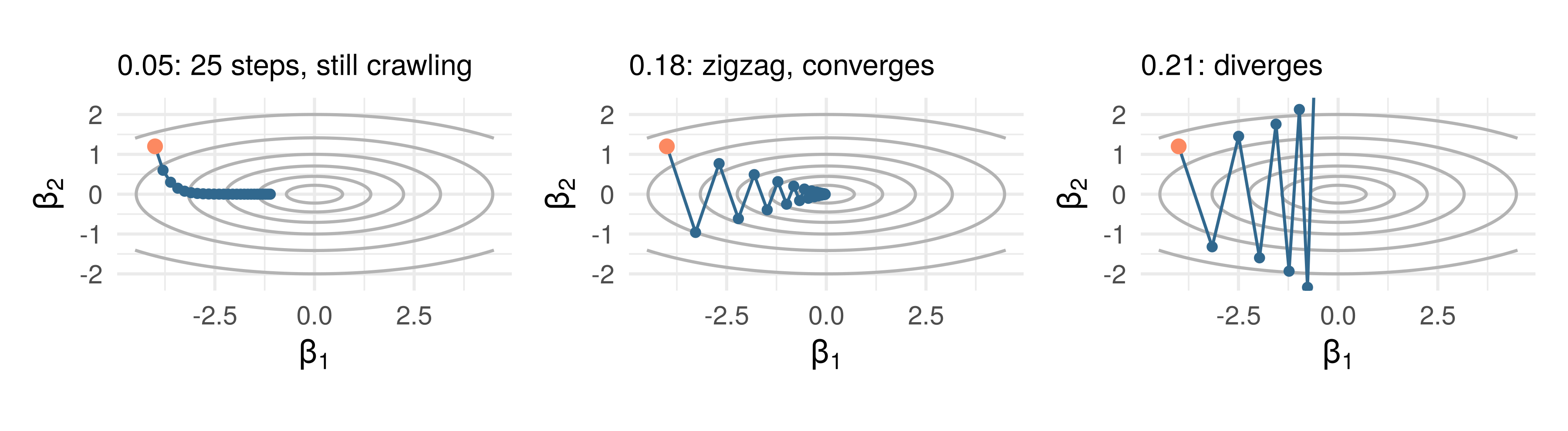
Across the valley the update multiplies \(\beta_2\) by \(1 - 10\gamma\): \(0.5\), \(-0.8\), \(-1.1\)

The quadratic case, exactly

One direction with curvature \(a > 0\): \(f(\beta) = \tfrac12 a\beta^2\), \(\nabla f = a\beta\), so

\[ \beta_{t+1} = \beta_t - \gamma a\beta_t = (1 - \gamma a)\,\beta_t, \qquad \beta_t = (1 - \gamma a)^t \beta_0 \]

Converges iff \(|1 - \gamma a| < 1\), i.e. \(0 < \gamma < 2/a\). The step \(\gamma = 1/a\) lands in one move

Several directions with curvatures \(a_1 \ge \dots \ge a_p\), one step size for all of them: \(\gamma < 2/a_1\) to converge, and the slowest direction shrinks like \((1 - \gamma a_p)^t\)

The largest curvature sets the safe step; the ratio \(a_1/a_p\), the shape of the valley, sets the speed. For least squares, \(\hat R_n(\beta) = \frac1n\|\mathbf y - \mathbf X\beta\|^2\), the \(a_j\) are the eigenvalues of \(2\mathbf X^\top\mathbf X/n\)

Beyond the quadratic: what could go wrong?

Taylor, to second order: for a smooth \(f\) and a small move \(\delta\), \(f(x + \delta) \approx f(x) + \nabla f(x)^\top\delta + \tfrac12\,\delta^\top \nabla^2 f(x)\,\delta\).

Take the step \(\delta = -\gamma\nabla f(x)\) and write \(g = \nabla f(x)\): \[ f(x - \gamma g) \approx f(x) \;\underbrace{-\; \gamma\,\|g\|^2}_{\text{always down}} \;\underbrace{+\; \tfrac12\gamma^2\, g^\top \nabla^2 f(x)\, g}_{\text{the curvature pushes back}} \]

In the quadratic case the curvature was a fixed number \(a\). Here it depends on where you stand, and the step is safe only if it is never too large

Curvature at most \(L\)

If the curvature in every direction is at most \(L\), the push-back is at most \(\tfrac12 L\gamma^2\|g\|^2\), and then \[ f(x - \gamma g) \lesssim f(x) - \gamma\big(1 - \tfrac12 L\gamma\big)\|g\|^2 \] The bracket is positive for \(\gamma < 2/L\) and the bound is best at \(\gamma = 1/L\): the quadratic case’s rule, in general

To make this a theorem we need “curvature at most \(L\)” without a second derivative. Say it about the gradient:

Assumption. \(\nabla f\) is \(L\)-Lipschitz: \(\|\nabla f(x) - \nabla f(y)\| \le L\,\|x - y\|\) for all \(x, y\)

For a quadratic with curvatures \(a_1 \ge \dots \ge a_p\) this holds with \(L = a_1\); for least squares, \(L = 2\lambda_{\max}(\mathbf X^\top\mathbf X)/n\)

Descent lemma

Descent lemma. If \(\nabla f\) is \(L\)-Lipschitz, then for every \(x\) \[ f\!\left(x - \tfrac1L\nabla f(x)\right) \le f(x) - \frac{\|\nabla f(x)\|^2}{2L} \] Every step of size \(1/L\) decreases \(f\), by at least the squared gradient over \(2L\).

The proof tidies the heuristic. The second-order term came from Taylor’s theorem; instead, integrate the gradient along the step, and let the Lipschitz bound do what the curvature bound did

Descent lemma, proof (1 of 2)

Write \(v = y - x\) for the step, so that \(y = x - \gamma\nabla f(x)\) means \(v = -\gamma\nabla f(x)\), and \(x_t = x + tv\) for the point a fraction \(t\) of the way along it, so that \(\|x_t - x\| = t\|v\|\)

\[ \begin{alignedat}{2} f(y) - f(x) &= \int_0^1 \nabla f(x_t)^\top v\, dt &\quad& \class{fragment}{\color{gray}\small\text{(a) along the step}} \\ &\class{fragment}{{}= \nabla f(x)^\top v + \int_0^1 \big[\nabla f(x_t) - \nabla f(x)\big]^\top v\, dt} && \class{fragment}{\color{gray}\small\text{(b) add and subtract}} \\ &\class{fragment}{{}\le \nabla f(x)^\top v + \int_0^1 \|\nabla f(x_t) - \nabla f(x)\|\,\|v\|\, dt} && \class{fragment}{\color{gray}\small\text{(c) Cauchy-Schwarz}} \\ &\class{fragment}{{}\le \nabla f(x)^\top v + \int_0^1 L\,t\,\|v\|^2\, dt} && \class{fragment}{\color{gray}\small\text{(d) Lipschitz}} \end{alignedat} \]

Descent lemma, proof (2 of 2)

\[ \begin{alignedat}{2} f(y) - f(x) &\le \nabla f(x)^\top v + \int_0^1 L\,t\,\|v\|^2\, dt &\quad& \\ &\class{fragment}{{}= \nabla f(x)^\top v + \tfrac{L}{2}\|v\|^2} && \class{fragment}{\color{gray}\small\text{(e) } \textstyle\int_0^1 t\, dt = \tfrac12} \\ &\class{fragment}{{}= -\gamma\|\nabla f(x)\|^2 + \tfrac{L}{2}\gamma^2\|\nabla f(x)\|^2} && \class{fragment}{\color{gray}\small\text{(f) } v = -\gamma\nabla f(x)} \\ &\class{fragment}{{}= -\gamma\big(1 - \tfrac12 L\gamma\big)\|\nabla f(x)\|^2} && \class{fragment}{\color{gray}\small\text{(g) collect}} \end{alignedat} \]

At \(\gamma = 1/L\) the right-hand side is \(-\|\nabla f(x)\|^2/2L\), which is the lemma. \(\blacksquare\)

For any \(0 < \gamma < 2/L\) the right-hand side is negative: every such step decreases \(f\), and the heuristic’s bound was right

Logistic regression by descent

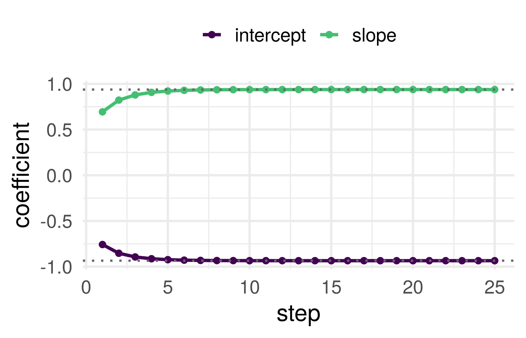
Chinstrap against Adelie from flipper length (standardized), penguins data, from \(\beta_0 = (0, 0)\), step \(\gamma = 4\)

Objective: \(\hat R_n(\beta) = -\ell(\beta)/n\). Gradient, from part 1: \(-\mathbf X^\top(\mathbf y - \mathbf p(\beta))/n\)

Same loop as least squares; only the gradient function changed. Dotted lines: glm’s answer

Curvature: the Hessian of \(\hat R_n\) is \(\frac1n\sum_i \hat p_i(1 - \hat p_i)x_ix_i^\top \preceq \mathbf X^\top\mathbf X/4n\), so \(L = 0.25\) here and \(2/L = 8\)

Optimization theory

\(f(u, v) = (u^2 - 1)^2 + v^2\). Compute the gradient at \((0, 0)\). Is \((0, 0)\) a minimum?

• If the loss function is convex many of these methods have guaranteed convergence to the global minimizer

• If the loss function is non-convex, we lose mathematical guarantees

  • Possible convergence to local minimizer, or to a saddle point like the one above (gradient zero, curvature \(-4\) one way and \(+2\) the other)

  • Local minimizers may be much worse than the best possible model…

  • Or they might not be!

Deep learning: to hell with convexity 🤠 “it just works”

Part 3: stochastic gradient descent

History: September 2012

60,000,000

parameters in the model that cut the ImageNet top-5 error to 15.3%, against 26.2% for the next best entry

Fitted in five to six days on two gaming graphics cards, by stochastic gradient descent. Nobody solved an equation

Krizhevsky, Sutskever and Hinton, “ImageNet classification with deep convolutional neural networks”, NeurIPS 2012

Computational complexity

• Second order methods, like Newton-Raphson, use second derivatives, i.e. inverting the \(p \times p\) Hessian matrix

• First order methods, like gradient descent, only require computing the \(p \times 1\) gradient vector

Many parameters \(\to\) prefer first order methods

What a step costs

	Operations	Once or per step?
Least-squares formula \((\mathbf X^\top\mathbf X)^{-1}\mathbf X^\top\mathbf y\)	about \(np^2 + p^3\)	once
One gradient-descent step	about \(np\)	per step
One step on a random batch of \(b\) rows	about \(bp\)	per step

\(n = 1{,}200{,}000\) images, \(p = 60{,}000{,}000\) parameters. Roughly how many operations is one full gradient? And one step on a batch of 128?

Coordinate descent

Update only one coordinate of \(\beta\) in each step

Cycle through coordinates until some convergence criteria is satisfied

Can combine with any strategy for univariate optimization – e.g. one-dimensional Newton’s method – treating other parameters as constants

Stochastic/random descent

• Instead of cycling through all coordinates in coordinate descent, just pick one randomly

• Instead of computing the gradient of the loss function on the entire dataset, compute it on a random sample

Pick one row \(I\) uniformly at random from \(\{1, \ldots, n\}\) and use its gradient \(\nabla\ell_I(\beta)\) in place of the average over all \(n\) rows. Commit: is it biased for the full gradient \(\nabla\hat R_n(\beta)\), yes or no?

The stochastic gradient is unbiased

With the data and \(\beta\) held fixed, only \(I\) is random, and by linearity of \(\nabla\), \(\mathbb E\) and \(\sum\), \[ \mathbb E_I\big[\nabla\ell_I(\beta)\big] = \sum_{i=1}^n \frac1n\,\nabla\ell_i(\beta) = \nabla\hat R_n(\beta) \]

Unbiased, whatever the data are. A batch of \(b\) rows drawn independently with replacement averages \(b\) such gradients: still unbiased, with variance \(\sigma^2(\beta)/b\), where \(\sigma^2(\beta)\) is the spread of the single-row gradients

Compute update using one randomly sampled observation, or a randomly sampled subset (“mini-batch SGD”)

Scale up more! Bigger data!

The step must shrink, but not too fast

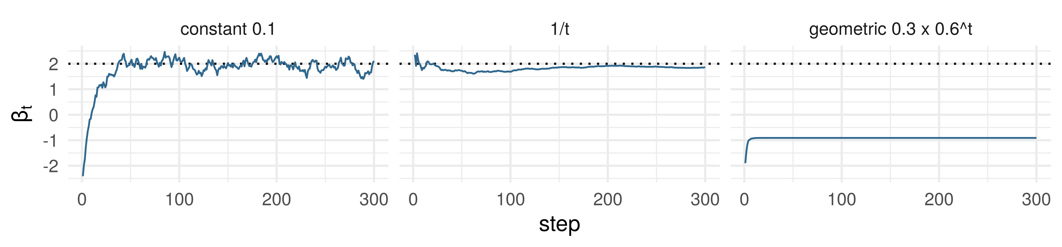
Simulated: one parameter, noisy gradient \((\beta - 2) + \text{noise}\), from \(\beta_0 = -3\). Target: 2

One of the three stalls short of the target for ever. Which, and why?

Without noise, a constant step below \(2/L\) is right. With noise the steps must shrink, \(\gamma_t \to 0\), but not too fast: \(\sum_t \gamma_t = \infty\) and \(\sum_t \gamma_t^2 < \infty\) (Robbins and Monro, 1951)

Constrained and non-smooth optimization

Constrained. Some optimization problems have constraints on the parameters. If a descent step takes us outside the constraint region: choose step sizes small enough to stay inside, or project the updated point to the nearest point inside the region

Non-smooth. If the loss function is not (everywhere) differentiable but still convex, e.g. absolute value: there is no gradient at a kink but there is a subgradient, any slope whose tangent line stays below the function. Take a step along one of those

Part 4: where the error comes from, this time

Choosing tuning parameters

e.g. number of predictors, flexibility for non-linear methods

Modeling assumption: smoothness

Version of simplicity/parsimony for flexible function classes

Linear functions are the smoothest

Smooth function classes: set of functions with some type of bound on second derivatives, for example

Cool math fact: can be related to sparsity by considering (rate of decay of) coefficients of function’s Fourier transform (smoother functions have sparser representations when written in a basis of sine functions, for example)

Discretize and fit sequentially

• Start with a grid of values for the tuning parameter
• Fit the model for each value in this grid
• Pick the best fit (visually, or based on loss function value, or…)

e.g. For the span or fraction \(s\) in local regression, try \(s \in \{ 0.1, 0.25, 0.5, 0.75, 0.9 \}\) and visualize the result

• Problem: When to stop increasing the complexity? (i.e. decreasing the smoothness). We’ll come back to this

Three functions

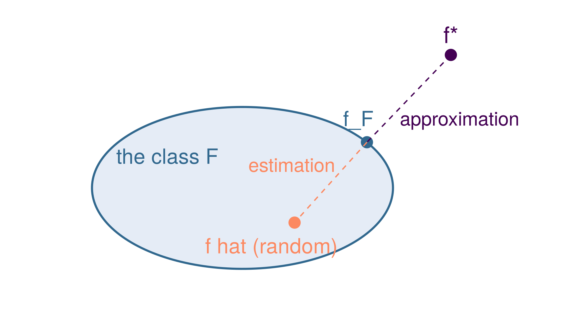
\(f^\star\): the best predictor of all, \(\arg\min_f R(f)\)

\(f_{\mathcal F}\): the best in the class, \(\arg\min_{f \in \mathcal F} R(f)\). Fixed once \(\mathcal F\) is chosen; not random

\(\hat f\): what the algorithm returns from the sample. Random, and in \(\mathcal F\)

Double \(n\). Which of the two dashed distances shrinks, and which does not know that \(n\) changed?

Bias and variance, again

Week 1, \(k\)-nearest neighbors: the expected squared error at a point is noise \(+\) bias\(^2\) \(+\) variance, with the bias set by the method and the variance falling with \(k\). Week 2, the optimal model theorem: \(R(f) - R(f^\star) = \mathbb E[(f^\star(X) - f(X))^2]\) for squared loss.

What we want small is the excess risk \(R(\hat f) - R(f^\star) \ge 0\): one number, for any loss

The class \(\mathcal F\) was chosen before the data arrived. So some of that number was decided then, by how far \(\mathcal F\) is from \(f^\star\); the rest depends on the sample. Split it there: add and subtract \(R(f_{\mathcal F})\)

\[ R(\hat f) - R(f^\star) = \big[R(\hat f) - R(f_{\mathcal F})\big] + \big[R(f_{\mathcal F}) - R(f^\star)\big] \]

Both brackets should be nonnegative: \(f_{\mathcal F}\) is the best in \(\mathcal F\), and \(\hat f\) is in \(\mathcal F\); \(f^\star\) is the best of all

Bias–variance decomposition, ERM form

Bias–variance decomposition, ERM form. \(\mathcal F\) a class of predictors with a best member \(f_{\mathcal F} = \arg\min_{f \in \mathcal F} R(f)\); \(\hat f \in \mathcal F\) the predictor an algorithm returns from the sample; \(f^\star = \arg\min_f R(f)\) over all predictors. Then \[ R(\hat f) - R(f^\star) = \underbrace{\big[R(\hat f) - R(f_{\mathcal F})\big]}_{\text{estimation}} + \underbrace{\big[R(f_{\mathcal F}) - R(f^\star)\big]}_{\text{approximation}}, \qquad \text{both terms} \ge 0 \]

Proof. The equation is adding and subtracting \(R(f_{\mathcal F})\). The first bracket is \(\ge 0\) because \(\hat f \in \mathcal F\) and \(f_{\mathcal F}\) minimizes \(R\) over \(\mathcal F\); the second because \(f^\star\) minimizes \(R\) over everything. \(\blacksquare\)

For squared loss, the optimal model theorem gives the approximation term a shape: \(R(f_{\mathcal F}) - R(f^\star) = \mathbb E[(f_{\mathcal F}(X) - f^\star(X))^2]\), the squared distance from the class to the truth

What the two terms do

Estimation error: random, depends on the sample, shrinks with \(n\), grows with \(\mathcal F\). Approximation error: fixed, zero only if \(f^\star \in \mathcal F\), shrinks with \(\mathcal F\). Week 1’s variance and bias, for any method that minimizes something over a class

The trade-off in numbers

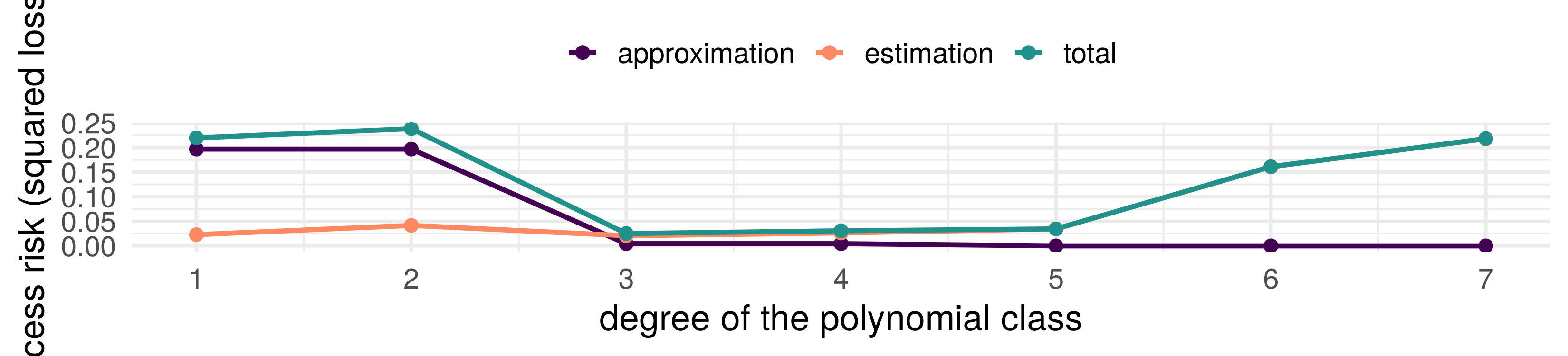
Simulated: \(f^\star(x) = \sin(2\pi x) + x/2\), \(X\) uniform on \([0, 1]\), noise sd \(0.4\), \(n = 40\); the class is the polynomials of degree \(d\), fitted by least squares; estimation is \(\mathbb E[(\hat f(X) - f_{\mathcal F}(X))^2]\) averaged over 200 samples

Double \(n\) to 80. Which curve moves, and which way?

No free lunch

No free lunch (stated). No method has lower error than every other on every distribution: for any learning method and any training size \(m\), on a domain with more than \(2m\) points there is a distribution for which a perfect predictor exists and the method’s expected error stays far from zero.

What it says: choosing a method is an assumption about the world, and the approximation term is its price. What it does not say: that methods are equally good on the problems we meet, or that an assumption is a flaw

In the week 1 seminar a line and \(k\) nearest neighbors often scored within a standard error of each other on gapminder. A fact about the methods, or about the data?

Part 5: stopping

Early stopping

Optimization time = complexity

• For many optimization algorithms the fitted model becomes more complex the longer the optimization algorithm runs

• e.g. the more steps of (stochastic) gradient descent used in combination with a flexible function class

• e.g. the more steps of forward stepwise (adding more predictor variables)

Idea: control model complexity by stopping the algorithm before convergence

This is early stopping – we’ll come back to it later

Stopping early

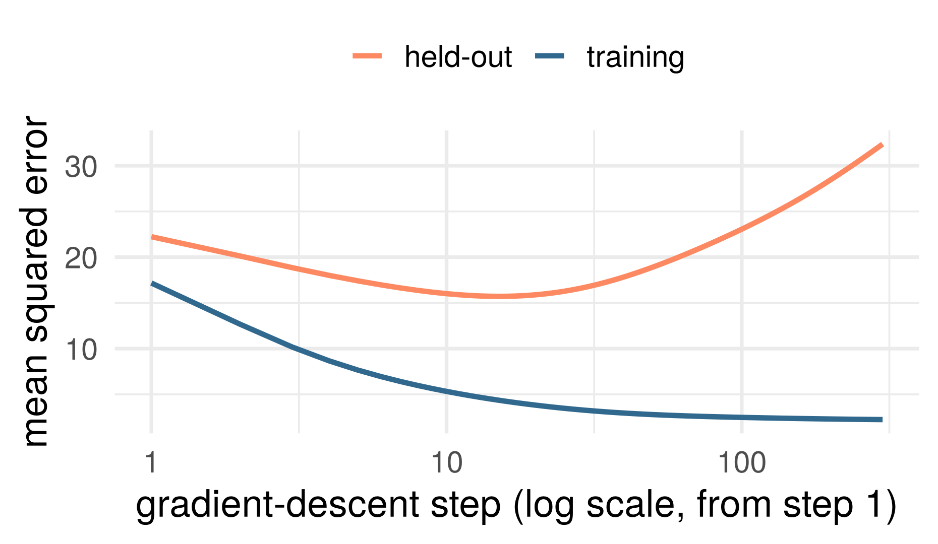
Simulated: least squares from \(\beta_0 = \mathbf 0\), \(n = 80\), \(p = 60\), noise sd 3, step \(1/2L\); held-out error on 2,000 new rows from the same model

Training error falls at every step. The held-out error falls, turns at step 15, and ends far above its minimum

The number of steps is a tuning parameter, like \(k\) or \(d\). Week 7 writes the penalty down, \(\hat R_n(\beta) + \lambda\|\beta\|^2\), with \(\lambda\) as the knob

Before the seminar

• This week: exercises 1 to 4 at the top of the notebook. The descent lemma and the ERM form of the bias–variance decomposition, both again with the slides closed; the second derivative of the logistic log-likelihood, finishing the Newton-Raphson exercise; and no free lunch on a finite domain

• In the seminar you write gradient descent once, as a function, and use it for least squares, then logistic regression, then with random batches

Conclusion: optimization in ML is a big topic

Strategies for specific problems

e.g. stepwise inclusion of variables, constraints, etc

Strategies for general loss/function classes

e.g. gradient methods, coordinate methods

Stopping at the right amount of complexity

Maybe the most important part! Next lecture