Last week: optimization, the general concepts and the methods that fit a model
This week: a few specific families of supervised models, each with its own functional structure, each introduced briefly. Every one of them gets more detail later in the course
Each family is a bet on the shape of \(f^\star\). To compare the bets we need one task
The task: 10,000 Spotify tracks
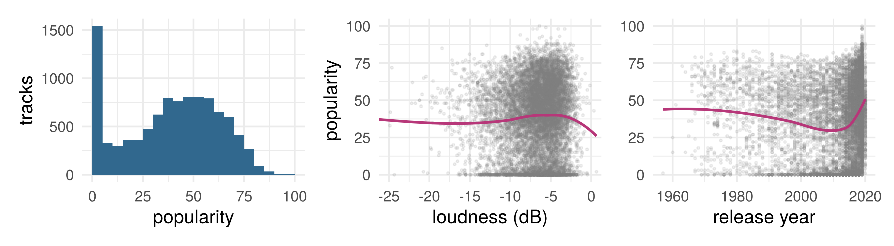
Predict a track’s popularity (Spotify’s score, 0 to 100) from ten audio features (danceability, energy, loudness, valence, tempo, …), its release year and its genre. Loss: squared error
10,000 tracks from playlists of six genres (data note); the 5,000 training tracks plotted. Their popularity has variance 565: the MSE of predicting the mean for everyone
Data split
Used for
How often
Training
fitting
as much as you like
Selection (books: validation)
choosing among fits: a method, its knob
as much as you like
Test, reserved
one number for the model you chose, with its standard error
once
ESL’s word for the third: a vault. Split once, at random, before looking (today 5,000, 2,000 and 3,000 tracks); refit the chosen model on training plus selection; open the vault once. A test set may score several competitors fixed in advance; nothing is chosen on it
The one rule for evaluation data: a row is fair game for scoring only if nothing about the model was chosen on it.
CTF competition: baselines
What we can fit so far, each a bet on \(f^\star\): least squares, a plane (every input a slope); logistic regression, a plane for the log-odds (for a label, not today); \(k\) nearest neighbors, a local average, its \(k\) the knob
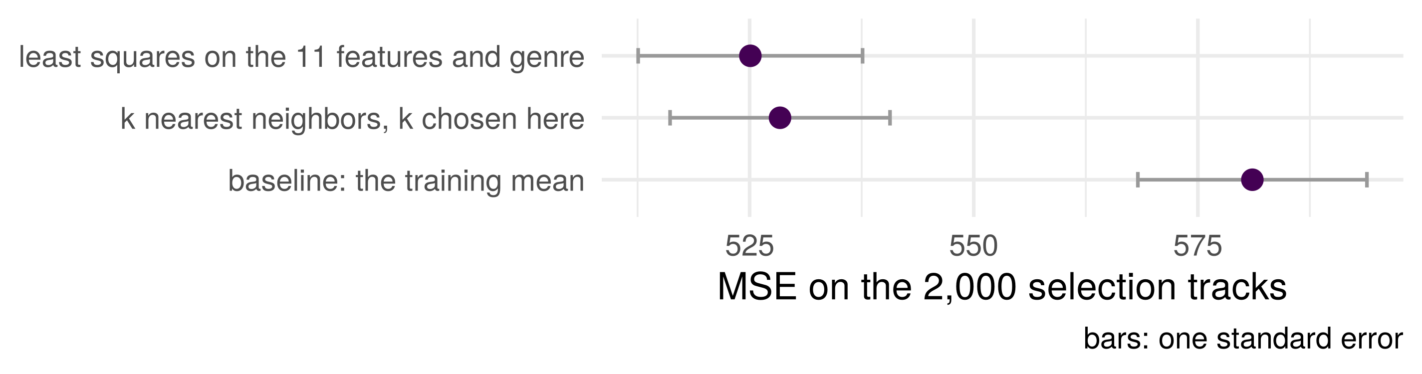
The local average (\(k = 100\)) and the plane, well within a standard error of each other. Can a different shape beat both? The test set stays shut
Tuning
Every candidate has a knob. Turn it, and the fit follows the data more or less closely
Candidate methods
Try several types of model, each with a different functional structure for \(f\):
Structure
Family
The knob
a plane, shrunk or sparse
ridge, lasso
\(\lambda\), how hard the penalty pulls
a sum of one-input curves
additive splines
\(J\), how many basis functions per input
rectangles with a constant in each
a tree
its depth
an average of many trees
a random forest
(defaults today)
a composition: a GLM of GLMs
a neural network
\(M\), how many hidden units
and tune each model so that it is the best version of its kind: every knob chosen on the selection tracks, as \(k\) was. Then compare the best of each kind
Part 2: ridge and lasso
Regularized (i.e. penalized) regression
Motivation: early stopping made the number of gradient-descent steps a knob that controlled how far the fit went. Can the knob be written into the objective instead?
For some penalty function \(\mathcal P_\lambda\), which depends on a tuning parameter \(\lambda\), the estimator
\[\hat \beta_\lambda = \arg \min_\beta \| \mathbf y - \mathbf X \beta \|^2_2 + \mathcal P_\lambda(\beta)\] is “regularized” or shrunk (shranken?) toward values that decrease the penalty. Often \(\mathcal P_\lambda = \lambda \| \cdot \|\) for some norm
Many ML methods are optimizing “loss + penalty”
Ridge (i.e. L2 penalized) regression
Originally motivated by problems where \(\mathbf X^T \mathbf X\) is uninvertible (or badly conditioned, i.e. almost uninvertible)
If \(p > n\) then this always happens
Least squares estimator is undefined or numerically unstable
For some constant \(\lambda > 0\), \[\text{minimize } \| \mathbf y - \mathbf X \beta \|^2_2 + \lambda \| \beta \|^2\]Shrinks coefficients \(\hat \beta\) toward 0
Larger coefficients are penalized more (squared penalty)
The ridge estimator
Set the gradient of \(\| \mathbf y - \mathbf X \beta \|^2 + \lambda \| \beta \|^2\) to zero (exercise 2): \[
(\mathbf X^T\mathbf X + \lambda I)\,\hat\beta_\lambda = \mathbf X^T\mathbf y
\]\[
\hat\beta_\lambda = (\mathbf X^T\mathbf X + \lambda I)^{-1}\mathbf X^T\mathbf y
\]
\(\mathbf X^T\mathbf X + \lambda I\) is invertible for every \(\lambda > 0\), whatever \(n\) and \(p\): one solution even when \(p > n\)
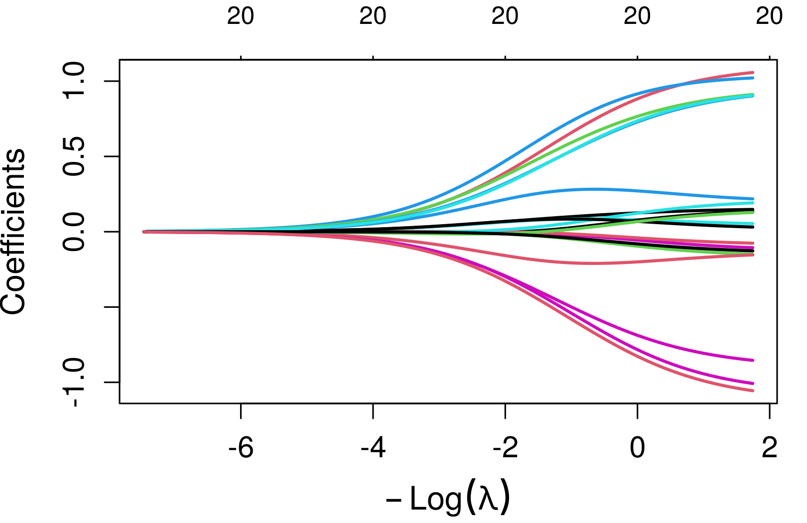
\(\lambda \to 0\): least squares (when it exists). \(\lambda \to \infty\): \(\hat\beta_\lambda \to \mathbf 0\)
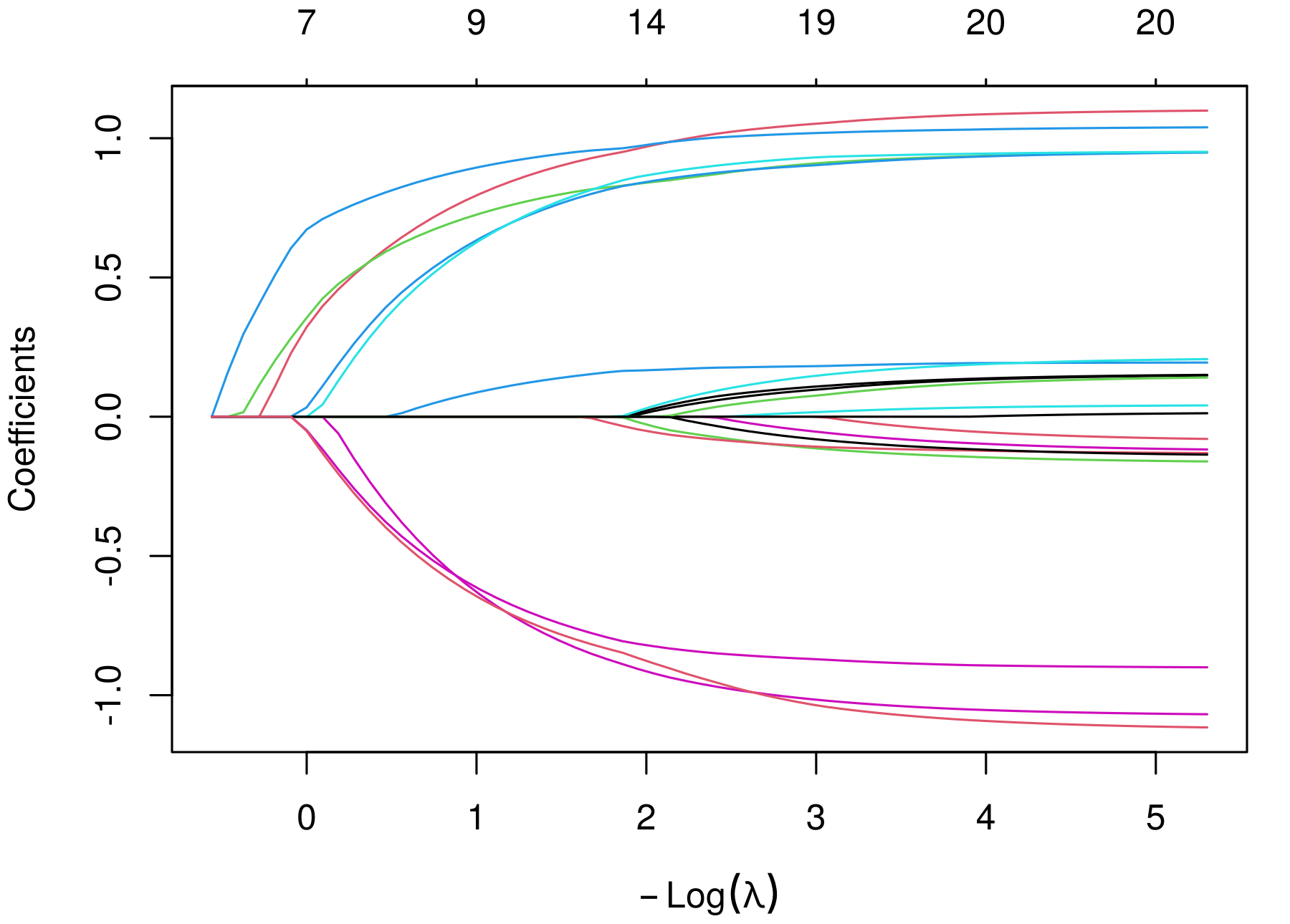
\(\hat\beta_\lambda\) against \(-\log\lambda\): the 16 standardized inputs (eleven numeric, five genre dummies), six named
Lasso vs ridge: L1 vs L2 norm penalties
A simple diff to remember lasso/ridge is via the penalty/constraint (1-norm instead of 2-norm). Lasso is
\[\text{minimize } \frac{1}{2n}\| \mathbf y - \mathbf X \beta \|_2^2 \text{ s. t. } \| \beta \|_1 \leq t\] where \(\| \beta \|_1 = \sum_{j=1}^p |\beta_j|\). Lagrangian form
\[\text{minimize } \frac{1}{2n} \| \mathbf y - \mathbf X \beta \|_2^2 + \lambda \| \beta \|_1\]
The lasso often gives estimates with many coefficients set to exactly zero
Lasso vs ridge: solution paths of \(\hat \beta\)
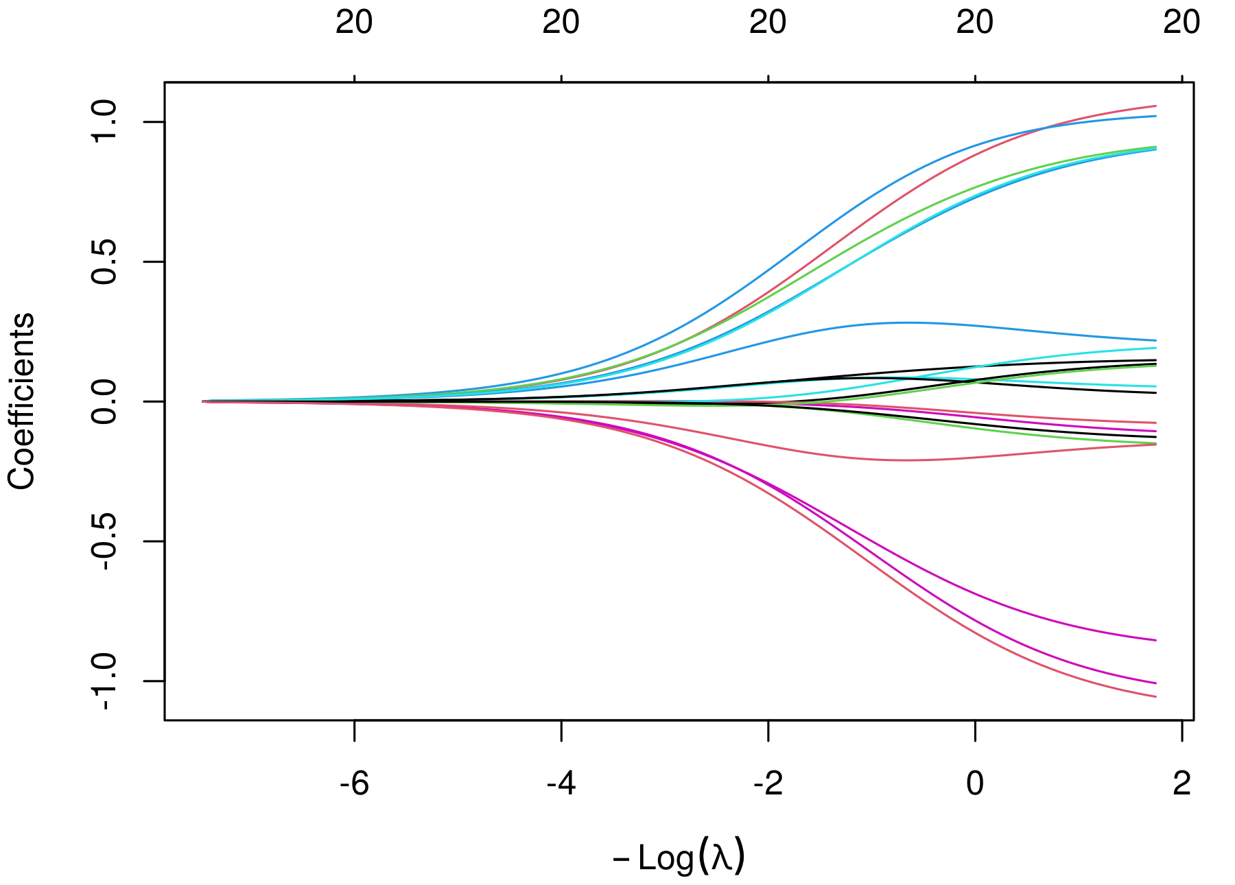
Spotify, the same 16 inputs, large \(\lambda\) on the left. The lasso’s coefficients are exactly zero over whole ranges of \(\lambda\) and enter one at a time; ridge’s are never zero
Part 3: additive models
Two ways to estimate a curve
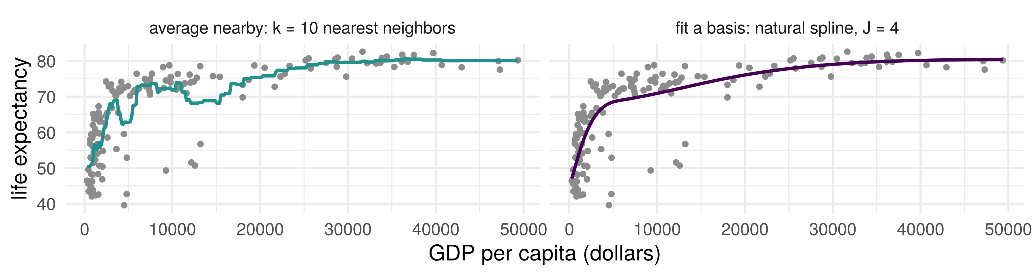
Life expectancy on GDP per capita, 142 countries in 2007 (no log this time). Two ways to turn a line into a curve
Average nearby (\(k\)-NN; a kernel weights by distance instead of cutting at \(k\)). Fit a basis: fixed curves, combined by least squares. We now focus on the second
A spline is regression on basis functions
A basis: fixed functions \(b_1(x), \ldots, b_J(x)\) of one input, combined by least squares: \[
f(x) = \beta_0 + \sum_{j=1}^J \beta_j\, b_j(x)
\] linear in \(\beta\): ns(gdpPercap, df = J) builds the \(J\) columns for lm()
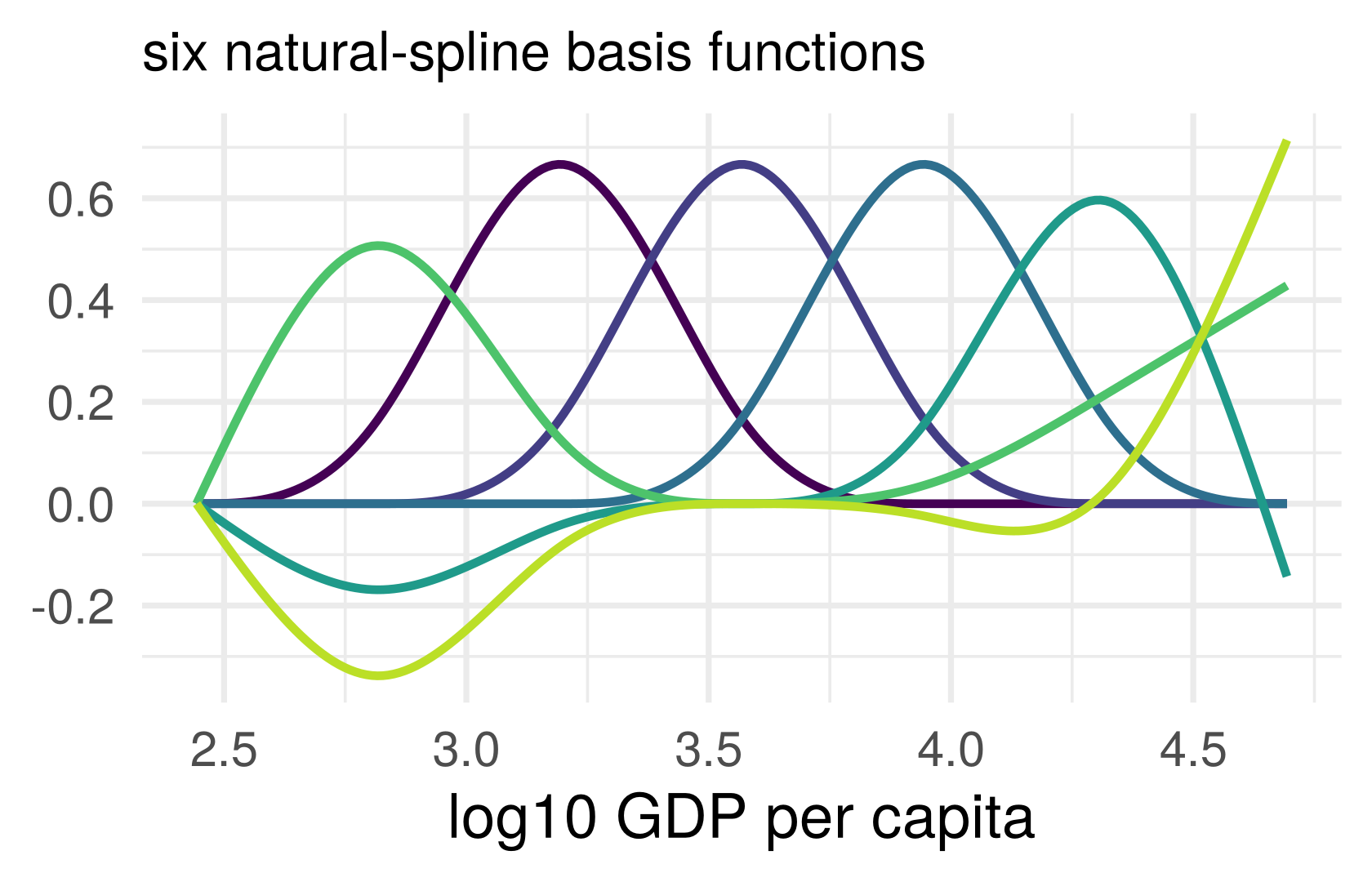
A natural cubic spline: cubic pieces joined smoothly at knots, linear beyond the ends. The basis functions are the bends the knots allow; lm adds \(\beta_0\)
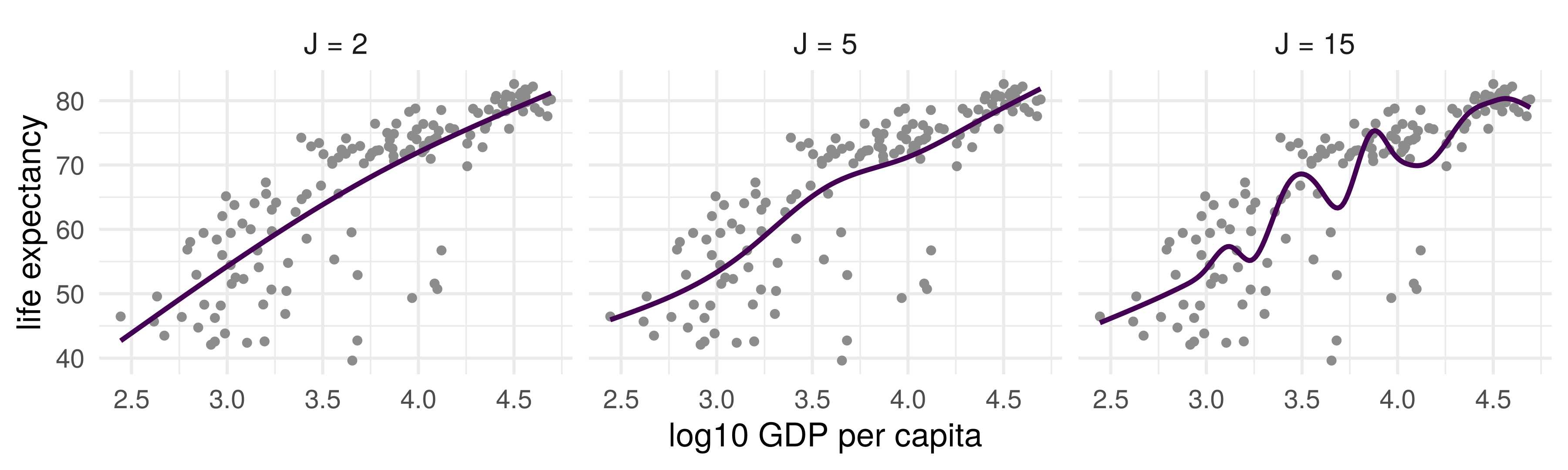
The basis size is the knob
Small \(J\): almost a line. Large \(J\): the curve follows the points, and at \(J = n\) it passes through every one (training error zero). Which \(J\)? The selection set, as for \(k\) and \(\lambda\). Later in the course: a penalty on wiggliness instead, with \(J\) as a ceiling
Additive modeling assumption
Linearity assumption: each predictor has a coefficient
Includes linear models as special case if \(f_j(\mathbf x_j) = \beta_j \mathbf x_j\)
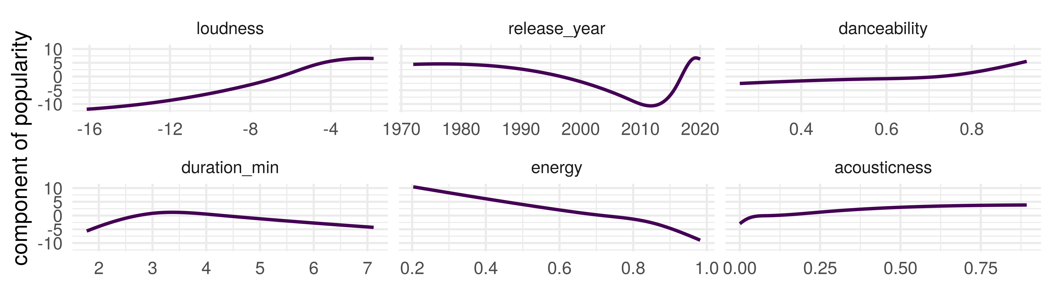
Today each \(f_j\) is a spline with \(J\) basis functions, so the whole model is one least-squares fit on \(pJ\) columns: lm(y ~ ns(x1, J) + ns(x2, J) + ...). The GAM in the reading is this model, with a link
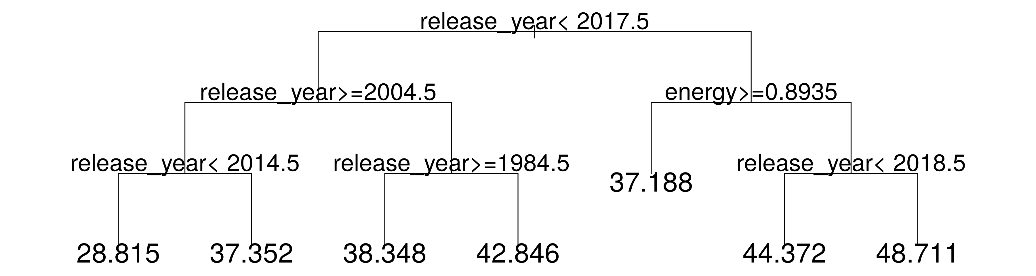
Left branch: yes. Leaves: mean popularity of the training tracks that reach them
Regression tree predictions
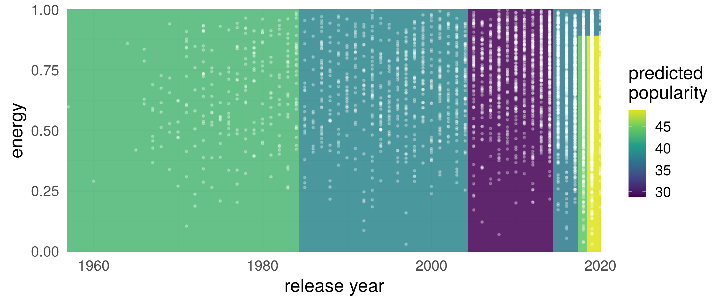
Each leaf is a rectangle with one value; the training tracks in white. Energy matters only on the right, from 2018 on: one leaf for the most energetic tracks, two below it
One predictor, every cutoff
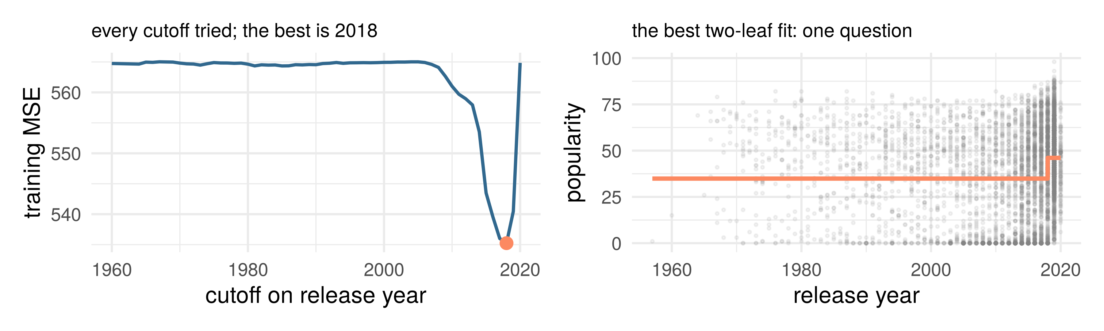
For one input: try every cutoff, predict each side’s mean, keep the cutoff with the smallest training MSE. One question, two leaves
Recursive rectangular splitting on predictors
“Stratification of the feature space”
Input: subset of data
  For each predictor variable x_j in subset
    Scan cutoff values to find the best split for x_j (last slide)
Output: the predictor and cutoff with the best improvement
Starting from the full dataset, compute the first split as above
Recurse: take the two subsets of data from each side of the split and plug them both back into the same function
Until some stopping rule prevents more splitting (today: a maximum depth, the tree’s knob; growing deep and pruning back comes later in the course)
A tree is unstable; a forest averages many
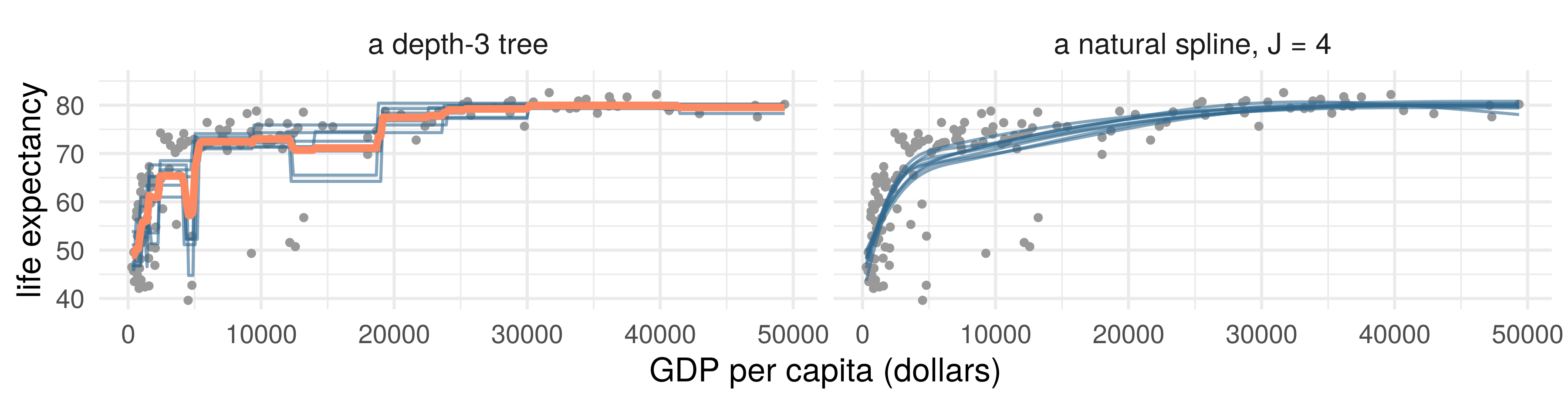
The 142 countries resampled eight times, one fit per resample (blue). The trees’ cutoffs jump with the sample; the splines barely move. Orange: the eight trees’ average
A random forest is a method that combines many trees into one model: hundreds of trees, each on a resample of the training rows, averaged (orange, with hundreds not eight). Today randomForest() with its defaults, no knob; details later in the course
Part 5: neural networks
A GLM of GLMs
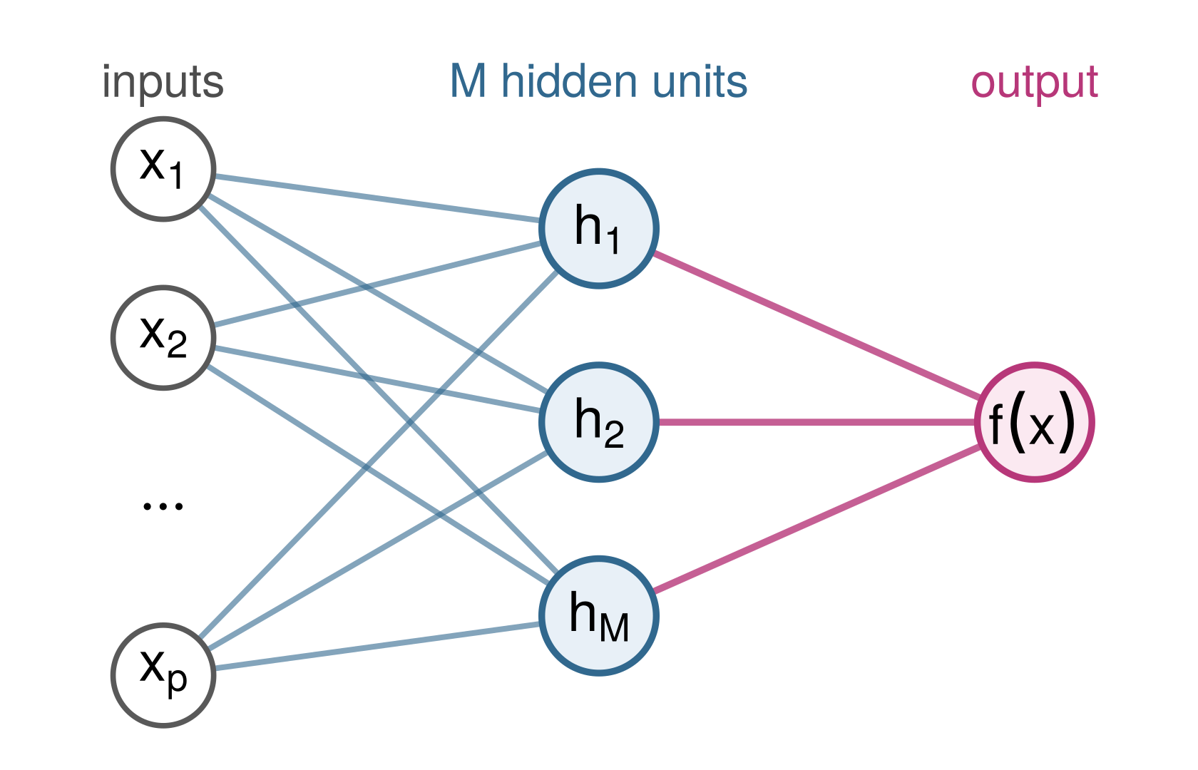
A GLM: the inverse link applied to a linear predictor, \(g^{-1}(\mathbf x^T\beta)\). Now iterate it
Hidden unit\(k\): a logistic regression of the inputs, with its own weights, \(h_k(x) = g^{-1}(w_{k0} + w_k^T x)\), \(g\) the logit link
Output: a linear regression on the hidden units, \(f(x) = \beta_0 + \sum_{k=1}^M \beta_k\, h_k(x)\) (logistic, for a label)
A GLM whose inputs are \(M\) GLMs. Iterate again: a deep network
Fitting and tuning a network
How it is fitted. All \(M(p + 1) + M + 1\) weights at once, by gradient-based optimization of a loss that is not convex: many valleys, with plateaus and saddles between them. Today’s fits: nnet(), a quasi-Newton method
The knob.\(M\), the number of hidden units, chosen on the selection tracks. Depth, and a penalty on the weights: later knobs. In R, nnet(size = M, linout = TRUE)
Part 6: which structure?
Comparison across three functional structures
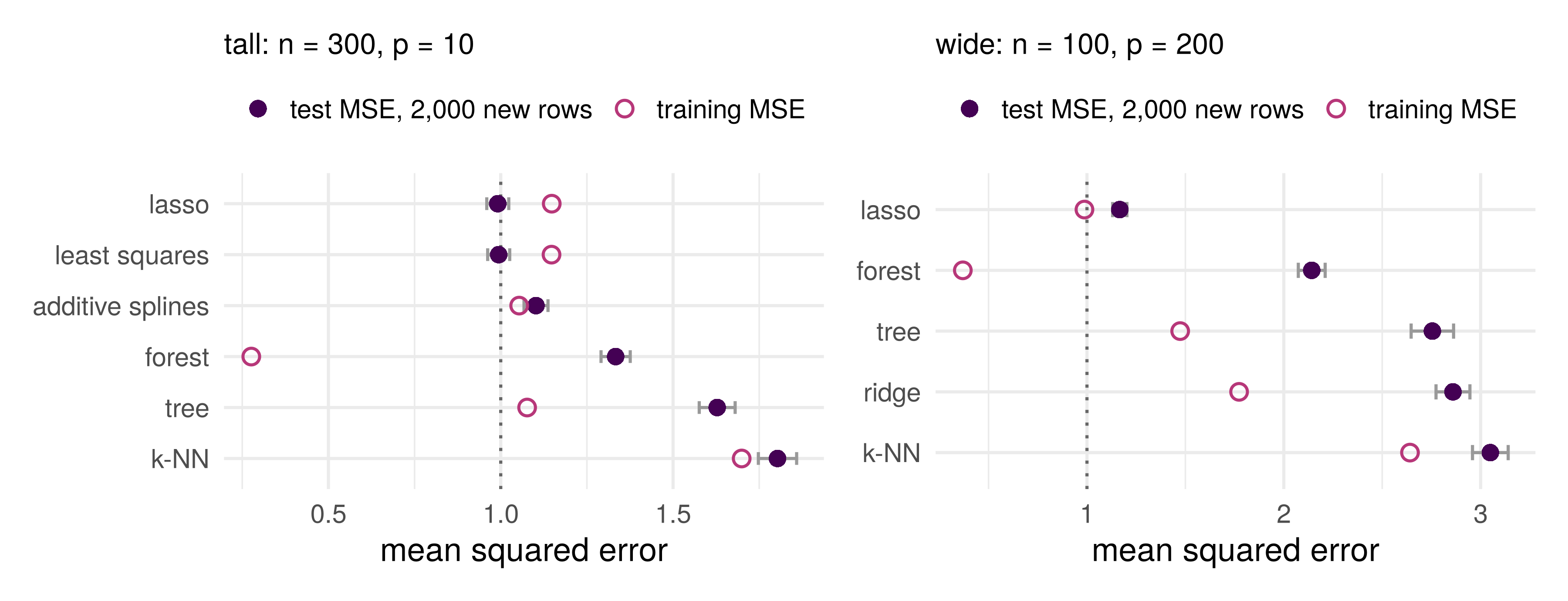
\(p = 10\) inputs on \([-1, 1]\), \(y = f^\star(x) + \varepsilon\), \(\sigma^2 = 1\). Three truths:
A, sparse linear:\(f^\star(x) = 2x_1 - 1.5x_2 + x_3\)
C, one step, two inputs at once:\(f^\star(x) = 4 \cdot \mathbf 1\{x_1 > 0,\ x_2 > 0\}\)
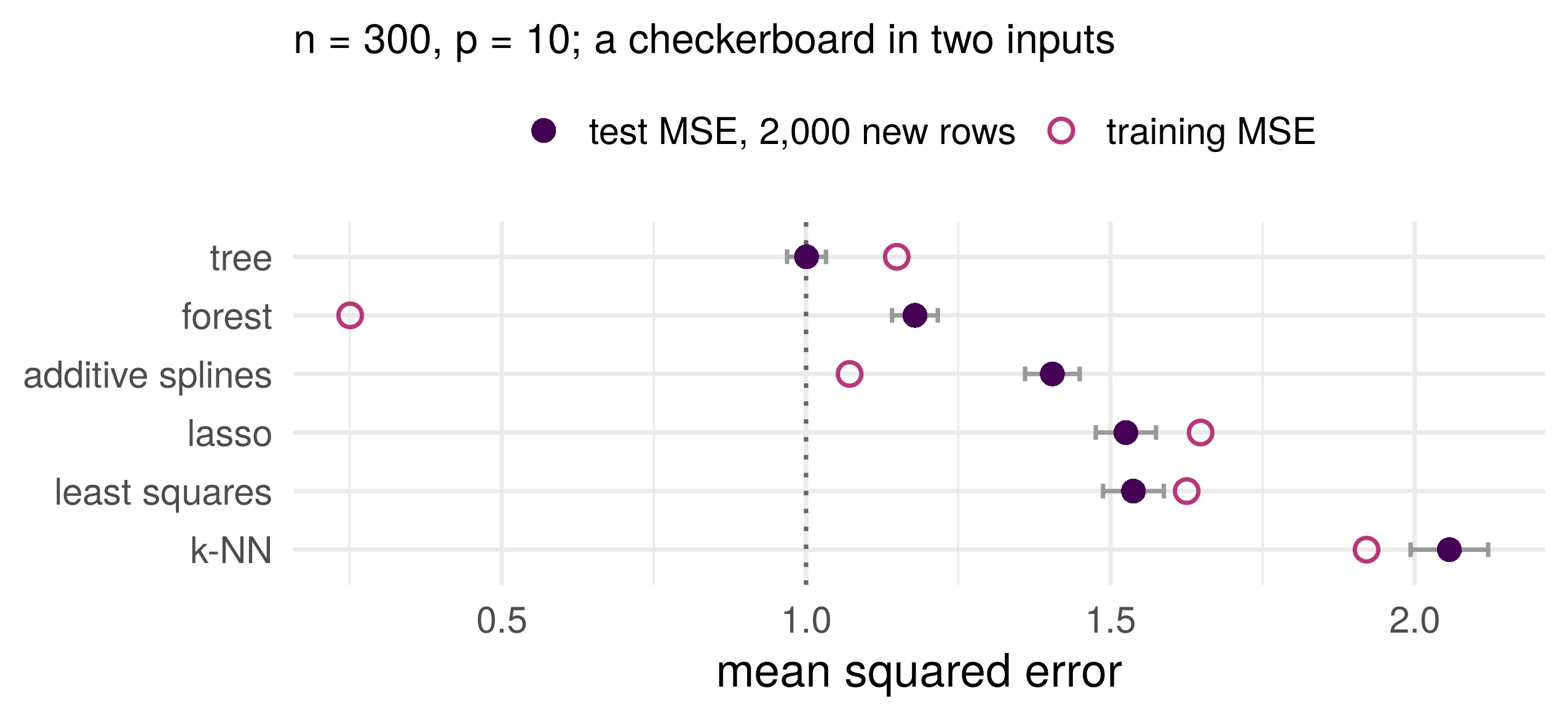
One task. 300 training, 100 selection, 2,000 test rows. Seven competitors: least squares; lasso (\(\lambda\)); \(k\)-NN (\(k\)); additive splines (\(J\)); a tree (depth); a forest; a network (\(M\)). Knobs chosen on the selection rows, refit on both, scored once
For each truth: which family wins, which loses, and why?
Truth A: sparse linear, tall and then wide
Dotted line: the noise variance, the smallest population MSE. For this sparse truth the lasso ties least squares when \(n \gg p\), and is far ahead of every other family when \(p > n\)
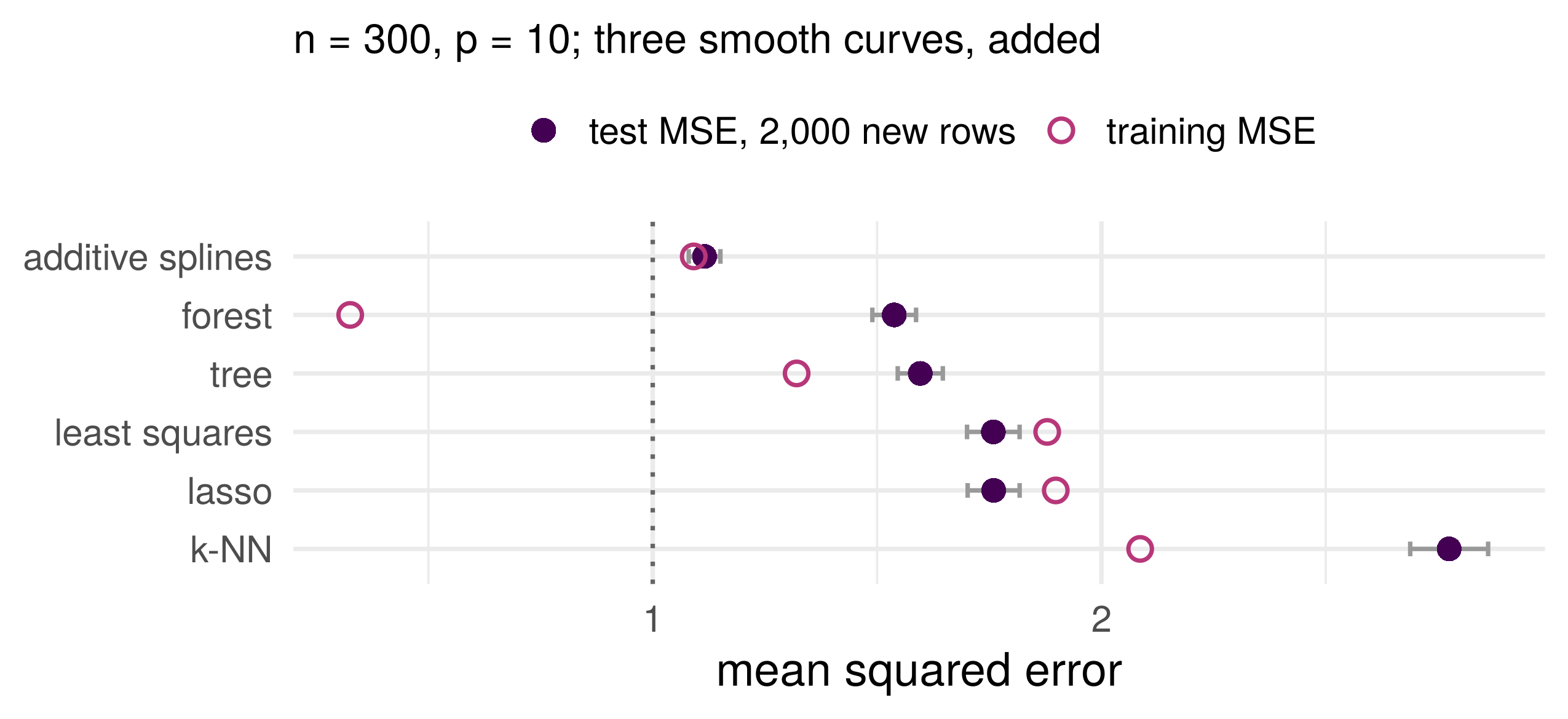
Truth B: additive smooth
The additive fit was built for this truth. A forest can bend, with rectangles; a plane cannot bend at all
Truth C: thresholds with an interaction
A sum of one-input functions can hold each input’s share of this step, two thirds of the signal at best, and not the product. Two questions in a row hold all of it
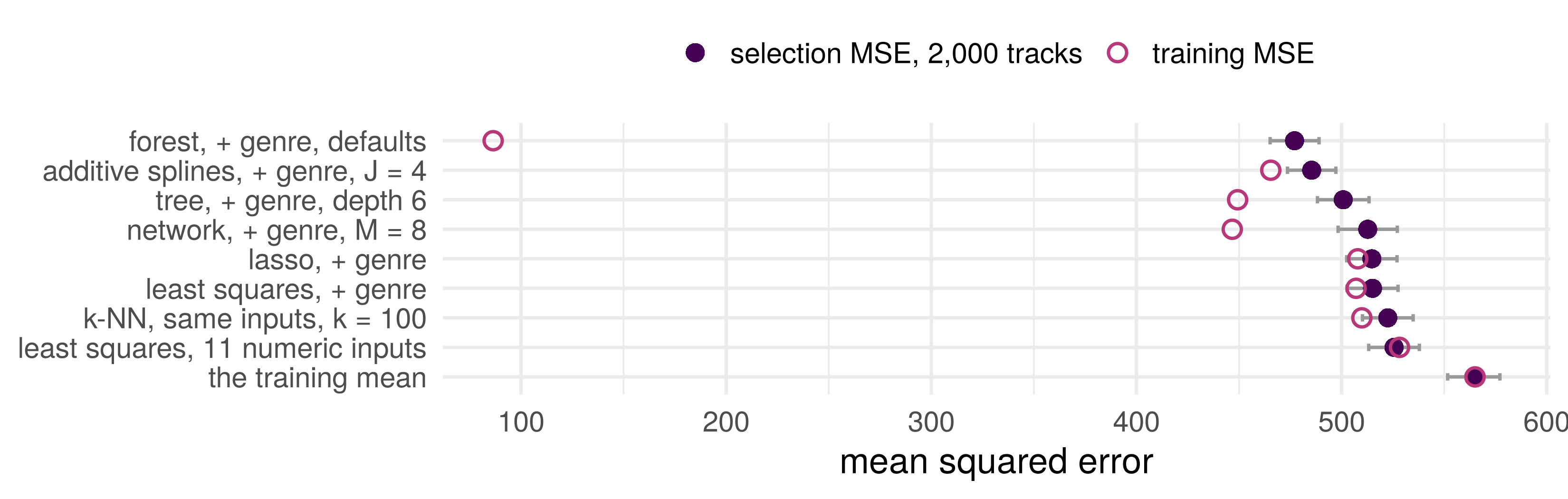
CTF competition: everyone on Spotify
Knobs chosen on the selection tracks, scored there. The forest and the additive splines lead, 30 to 40 below the plane with the same inputs; the forest’s training score is 86. The vault stays shut: the seminar refits and opens it once
Four dimensions, not one
Axis
The question about \(f^\star\)
Who bets which way
wide or tall
how \(p\) compares with \(n\)
least squares needs full column rank for one fit; the additive fit and a network overfit when \(n\) is small; ridge and the lasso fit at any \(p\)
sparse or dense
how many inputs matter
the lasso bets few; least squares and ridge spread the fit over all; a forest tolerates idle inputs, \(k\)-NN is hurt by them
smooth or discontinuous
how \(f^\star\) moves with each input
splines, \(k\)-NN and networks bet smooth; trees bet on steps
additive or interactive
whether inputs act separately
the additive fit bets separately; trees, forests, \(k\)-NN and networks allow interactions
Four separate questions, not one scale from simple to complex. A family is a bet on the answers. A selection set shows which bet did best on these data
Curse of dimensionality: \(k\)-NN last on truths A and B, seven idle inputs. No free lunch theorem: no family won every truth, and none can.
Training error and risk
On most rows of the leaderboards the training MSE sat below the test or selection MSE; on a few it sat above. Luck, or a law?
Training data i.i.d. from the population; a class \(\mathcal F\) fixed before the data; \(f_{\mathcal F}\) the best in \(\mathcal F\) (smallest \(R\)); \(\hat f\) the empirical risk minimizer (smallest \(\hat R_n\) over \(\mathcal F\))
Three numbers: \(\mathbb E[\hat R_n(\hat f)]\), \(R(f_{\mathcal F})\), \(\mathbb E[R(\hat f)]\). Put them in order, and write down what you used.
Optimism theorem
A function fixed before the data has an unbiased training error; \(\hat f\) was chosen to make its own small, and cannot beat \(f_{\mathcal F}\) on the population
Training data i.i.d.; \(\mathcal F\) fixed before the data; \(\hat f\) the empirical risk minimizer over \(\mathcal F\); \(f_{\mathcal F}\) the best in \(\mathcal F\) (risks finite, minimizers exist). Then \[
\mathbb E\big[\hat R_n(\hat f)\big] \;\le\; R(f_{\mathcal F}) \;\le\; \mathbb E\big[R(\hat f)\big]
\]
Training error underestimates the risk: on average it is below the best risk the class can reach, and the fitted model’s risk above it. A test set estimates \(R(\hat f)\); its average is the right end.
Proof: exercise 1
Before the seminar
This week: exercises 1 and 2 at the top of the notebook. The optimism theorem’s proof, three lines with numbered hints; and ridge’s normal equations, with why \(\mathbf X^T\mathbf X + \lambda I\) is invertible
In the seminar: the Spotify task with every family. Each knob chosen on the selection tracks, then the vault opened once for the leaderboard
Conclusion
Each family is a bet on the shape of \(f^\star\)
A plane, a sparse plane, a sum of curves, a set of rectangles, an average of many, a composition. Four questions about the world decide which bet pays
The data split decides what you may believe
Fit on the training rows, tune on the selection rows, open the test set once
Training error underestimates risk
Optimistic on average for every minimizer over a fixed class