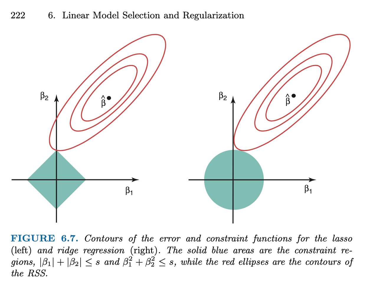
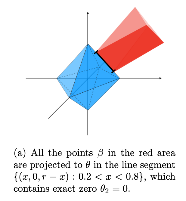
class: top, left, title-slide # Machine learning ## Lasso regression ### Joshua Loftus --- class: inverse <style type="text/css"> .remark-slide-content { font-size: 1.2rem; padding: 1em 4em 1em 4em; } </style> # Lasso regression #### Comparison to ridge regression #### Sparse models are more interpretable #### Optimality and degrees of freedom for lasso ## Inference #### ML/optimization finds the "best" model #### But is the best model actually good? --- class: inverse, center, middle # Interpretable ## high-dimensional regression ### with the lasso --- ### Lasso vs ridge - Generate some fake data from a linear model - Introduce lasso by comparison to ridge ```r library(glmnet) library(plotmo) # for plot_glmnet n <- 100 p <- 20 X <- matrix(rnorm(n*p), nrow = n) beta = sample(c(-1,0,0,0,1), p, replace = TRUE) Y <- X %*% beta + rnorm(n) lasso_fit <- glmnet(X, Y) ridge_fit <- glmnet(X, Y, alpha = 0) which(beta != 0) ``` ``` ## [1] 2 4 9 12 16 17 18 20 ``` Only 8 of the 20 variables have nonzero coefficients --- ### Lasso vs ridge: solution paths of `\(\hat \beta\)` .pull-left[ ```r plot_glmnet(ridge_fit, s = cv_ridge$lambda.1se) ``` <img src="06-2-lasso_files/figure-html/unnamed-chunk-3-1.png" width="504" /> ] .pull-right[ ```r plot_glmnet(lasso_fit, s = cv_lasso$lambda.1se) ``` <img src="06-2-lasso_files/figure-html/unnamed-chunk-4-1.png" width="504" /> ] --- ### Lasso vs ridge: L1 vs L2 norm penalties A simple `diff` to remember lasso/ridge is via the penalty/constraint (1-norm instead of 2-norm). Lasso is `$$\text{minimize } \frac{1}{2n}\| \mathbf y - \mathbf X \beta \|_2^2 \text{ s. t. } \| \beta \|_1 \leq t$$` where `$$\| \beta \|_1 = \sum_{j=1}^p |\beta_j|$$` Lagrangian form `$$\text{minimize } \frac{1}{2n} \| \mathbf y - \mathbf X \beta \|_2^2 + \lambda \| \beta \|_1$$` --- ## Lasso vs ridge: sparsity of solutions - For both ridge and lasso - Choose `\(\lambda\)` with cross-validation - Fit model on full data at the chosen `\(\hat \lambda\)` - Look at the estimate `\(\hat \beta\)` values... ```r cv_lasso <- cv.glmnet(X, Y) coef_lasso <- coef(lasso_fit, s = cv_lasso$lambda.1se) cv_ridge <- cv.glmnet(X, Y, alpha = 1) coef_ridge <- coef(ridge_fit, s = cv_ridge$lambda.1se) ``` Note: `lambda.1se` larger `lambda.min` `\(\to\)` heavier penalty --- ## Lasso vs ridge: sparsity of solutions ``` ## variable true_beta beta_hat_lasso beta_hat_ridge ## 1 1 0 0.0000 0.148 ## 2 2 1 0.9282 1.057 ## 3 3 0 0.0000 -0.149 ## 4 4 1 0.9558 1.021 ## 5 5 0 0.0000 0.054 ## 6 6 0 0.0000 -0.106 ## 7 7 0 0.0000 0.135 ## 8 8 0 0.0000 -0.076 ## 9 9 1 0.8165 0.911 ## 10 10 0 0.1529 0.218 ## 11 11 0 0.0000 0.192 ## 12 12 -1 -0.8508 -1.007 ## 13 13 0 0.0000 0.031 ## 14 14 0 -0.0052 -0.154 ## 15 15 0 0.0000 0.128 ## 16 16 1 0.7997 0.902 ## 17 17 1 0.8141 0.905 ## 18 18 -1 -0.7767 -0.854 ## 19 19 0 0.0000 -0.127 ## 20 20 -1 -0.8167 -1.056 ``` --- <img src="06-2-lasso_files/figure-html/unnamed-chunk-7-1.png" width="70%" /> True values are solid black dots, lasso estimates are hollow red circles, ridge estimates are blue crosses --- ### High dimensional example <img src="06-2-lasso_files/figure-html/unnamed-chunk-11-1.png" width="76%" /> --- <img src="06-2-lasso_files/figure-html/unnamed-chunk-12-1.png" width="90%" /> --- class: inverse # Lasso: cool or extremely cool? - High-dimensional: `\(p > n\)` means we can't fit OLS But all is not lost! Penalized regression to the rescue - True model is sparse Only 21 of 200 variables have nonzero coefficients - Ridge estimates are dense All coefficients nonzero 😰 - Lasso estimates are sparse Nonzero estimates largely coincide with true model 😎 --- ## Lessons about sparsity ### Solving otherwise impossible problems *Curse of dimensionality* / NP-hard optimization (best subsets) / unidentifiable statistical estimation / overfitting vs generalization Need special mathematical structure like sparsity to make things tractable ### Sparsity helps with interpretation Easier to interpret 38 nonzero coefficients than all 200 --- ### Sparse models are more interpretable Usual linear model interpretation of coefficients If the conditional expectation function (CEF) is linear `$$f(\mathbb x) = \mathbb E[\mathbf Y | \mathbf X = \mathbf x] = \beta_0 + \sum_{j=1}^p \beta_j x_j$$` Then `$$\hat \beta_j \approx \frac{\partial}{\partial x_j} \mathbb E[\mathbf Y | \mathbf X = \mathbf x]$$` "Change in CEF *holding other variables constant*" Small set of **other variables** `\(\to\)` easy (human) understanding --- ### Why are lasso estimates sparse? - **Lagrangian form** `$$\hat \beta_{\text{lasso}}(\lambda) = \arg\min_\beta \frac{1}{2n} \| \mathbf y - \mathbf X \beta \|_2^2 + \lambda \| \beta \|_1$$` - **Constrained form** `$$\hat \beta_{\text{lasso}}(t) = \arg\min_\beta \frac{1}{2n}\| \mathbf y - \mathbf X \beta \|_2^2 \text{ s. t. } \| \beta \|_1 \leq t$$` Level sets `\(\{ \beta : \| \mathbf y - \mathbf X \beta \|_2^2 = \text{const.} \}\)` are **ellipsoids** Level sets: `\(\{ \beta : \| \beta \|_1 = t \}\)` are **diamond thingies** (i.e. "cross polytope" or `\(L^1\)` ball) --- ## KKT optimality conditions Constrained optimization in multivariate calculus: - Switch to lagrangian form - Check stationary points (vanishing gradient) - Check boundary/singularity points - Verify feasibility (constraints satisfied) (Exam note: problems may use multivariate calculus like this) The [Karush-Kuhn-Tucker](https://en.wikipedia.org/wiki/Karush%E2%80%93Kuhn%E2%80%93Tucker_conditions) (KKT) conditions generalize these, useful for analysis of constrained optimization problems (i.e. almost all ML methods) -- more advanced, **not examinable** Recall: optimizer occurs at point of intersection between level sets of constraints and level sets of objective --- #### Why are lasso solutions sparse? ISLR Figure 6.7  --- ## Why are lasso solutions sparse? The `\(L^1\)` ball in `\(\mathbb R^p\)` `\(\{ x : \| x \|_1 = \text{const} \}\)` contains - `\(2p\)` points that are 1-sparse `\(x_j = \pm 1\)`, `\(x_{-j} = 0\)` - `\(\binom{p}{k} 2^k\)` points `\(k\)`-sparse with elements `\(\pm k^{-1}\)` - Higher dimensional edges/faces spanning (some) sets of these points, etc - Each of these is sparse, i.e. many coordinates are 0 -- The ellipsoid `\(\| \mathbf y - \mathbf X \beta \|_2^2 = \text{const}\)` *probably* intersects one of these *sharp parts of the diamond thingies* Solution to optimization problem is an intersection point --- ## Why are lasso solutions sparse? .pull-left[ At the point of intersection of the ellipse and the `\(L^1\)` ball, the normal vector of the ellipse has to be in the *normal cone* of the `\(L^1\)` ball (at the same point) Another intuition: consider projecting to the nearest point on the surface of the `\(L^1\)` ball (see figure) ] .pull-right[  From Figure 1 in [Xu and Duan (2020)](https://arxiv.org/abs/2006.01340) ] --- ### Optimality: stationary points - Of the **OLS** objective (uncorrelated residuals) $$ \frac{1}{n} \mathbf X^T ( \mathbf X \hat \beta - \mathbf y) = 0 $$ - For **ridge** (larger `\(|\hat \beta_j|\)` have larger resid. covariance) $$ \frac{1}{n} \mathbf X^T ( \mathbf X \hat \beta - \mathbf y) = - 2\lambda \hat \beta $$ - For **lasso** (resid. |covar| = `\(\lambda\)` if `\(\hat \beta_j \neq 0\)` and `\(\leq \lambda\)` otherwise) $$ \frac{1}{n} \mathbf X^T ( \mathbf X \hat \beta - \mathbf y) = - \lambda \text{ sign}(\hat \beta) $$ *Lasso treats predictors more "democratically"* --- ## Optimism / generalization gap **Recall**: for some `\(\text{df}(\hat f) > 0\)` (depends on problem/fun. class) `$$\Delta = \mathbb E_{Y|\mathbf x_1, \ldots, \mathbf x_n}[R(\hat f) - \hat R(\hat f)] = \frac{2\sigma^2_\varepsilon}{n} \text{df}(\hat f) > 0$$` #### Fairly general case For many ML tasks and fitting procedures `$$\text{df}(\hat f) = \frac{1}{\sigma^2_\varepsilon} \text{Tr}[ \text{Cov}(\hat f (\mathbf X), \mathbf y) ] = \frac{1}{\sigma^2_\varepsilon} \sum_{i=1}^n \text{Cov}(\hat f (\mathbf x_i), y_i)$$` --- ### Degrees of freedom: classic regression case If `\(\hat f\)` is linear with deterministic set of `\(p\)` predictors (or `\(p\)` basis function transformations of original predictors) then $$ \text{df}(\hat f) = p, \text{ so } \Delta = 2 \sigma^2_\varepsilon \frac{p}{n} $$ But if we do model/variable selection and use the data to choose `\(\hat p\)` predictors then *usually* $$ \text{df}(\hat f) > \hat p $$ And the more optimization / larger search this involves, it becomes more likely that $$ \text{df}(\hat f) \gg \hat p $$ --- ### Degrees of freedom: lasso case The "0-norm" (not really a norm) counts sparsity `$$\| \beta \|_0 = \sum_{j=1}^p \mathbf 1_{\beta_j \neq 0} = | \{ j : \beta_j \neq 0 \} |$$` e.g. for OLS with deterministic choice of variables `$$\text{df}(\hat \beta_\text{OLS}) = \| \hat \beta_\text{OLS} \|_0$$` **Surprisingly**, under fairly weak conditions on `\(\mathbf X\)` (columns in "general position"), for the lasso solution `\(\hat \beta(\lambda)\)` `$$\mathbb E[\| \hat \beta_\text{lasso}(\lambda) \|_0] = \text{df}(\hat \beta_\text{lasso}(\lambda))$$` **Solution sparsity is unbiased estimate of df** - like OLS case --- class: inverse # Choosing `\(\lambda\)` for lasso - Could use degrees of freedom combined with AIC, BIC, etc - Most commonly people use **cross-validation** ### Important note .pull-left[ `\(\hat \beta_\text{lasso}(\lambda)\)` at fixed `\(\lambda \quad \quad\)` vs ] .pull-right[ `\(\hat \beta_\text{lasso}(\hat \lambda)\)` at data-chosen `\(\hat \lambda\)` ] Different in general! e.g. Theoretical results about first may not apply to the second --- ## plot(cv.glmnet) and plot(glmnet) .pull-left[ ```r cv_fit <- cv.glmnet(X, Y) plot(cv_fit) ``` <img src="06-2-lasso_files/figure-html/unnamed-chunk-13-1.png" width="504" /> ] .pull-right[ ```r plot_glmnet(lasso_fit, s = cv_fit$lambda.1se) ``` <img src="06-2-lasso_files/figure-html/unnamed-chunk-14-1.png" width="504" /> ] --- class: inverse, middle, center # Inference ## for high-dimensional regression We have used regularization to avoid overfitting But this results in bias, e.g. `\(\| \hat \beta \|\)` smaller than true `\(\| \beta \|\)` Inference must correct for this somehow --- ## Approaches to inference - Debiased inference - Selective inference - Post-selection inference - Stability selection `R` packages for some of these Topic for future study? 😁 --- ## One example ```r set.seed(1) n <- 100; p <- 200 X <- matrix(rnorm(n*p), nrow = n) beta = sample(c(-1, rep(0, 20), 1), p, replace = TRUE) Y <- X %*% beta + rnorm(n) ``` Cross-validation plot (next slide) ```r beta_hat <- coef(lasso_fit, s = cv_lasso$lambda.min)[-1] vars <- which(beta_hat != 0) vars ``` ``` ## [1] 24 34 43 90 111 125 156 168 ``` **Idea**: since `\(\hat \beta\)` is biased by penalization, how about refitting OLS (unpenalized) using only these variables? --- <img src="06-2-lasso_files/figure-html/unnamed-chunk-18-1.png" width="504" /> --- ```r summary(lm(Y ~ X[,vars]-1)) ``` ``` ## ## Call: ## lm(formula = Y ~ X[, vars] - 1) ## ## Residuals: ## Min 1Q Median 3Q Max ## -1.598 -0.238 0.212 0.772 2.609 ## ## Coefficients: ## Estimate Std. Error t value Pr(>|t|) ## X[, vars]1 0.2373 0.0871 2.72 0.00771 ** ## X[, vars]2 -0.1335 0.0806 -1.66 0.10079 ## X[, vars]3 -0.1677 0.0768 -2.18 0.03160 * ## X[, vars]4 -0.3063 0.0817 -3.75 0.00031 *** ## X[, vars]5 -0.1351 0.0797 -1.70 0.09330 . ## X[, vars]6 0.1881 0.0808 2.33 0.02209 * ## X[, vars]7 -0.1481 0.0816 -1.81 0.07279 . ## X[, vars]8 -0.1530 0.0807 -1.90 0.06121 . ## --- ## Signif. codes: 0 '***' 0.001 '**' 0.01 '*' 0.05 '.' 0.1 ' ' 1 ## ## Residual standard error: 0.81 on 92 degrees of freedom ## Multiple R-squared: 0.375, Adjusted R-squared: 0.32 ## F-statistic: 6.89 on 8 and 92 DF, p-value: 4.5e-07 ``` --- ## Looks good, time to publish! - Sparse, interpretable model - Some significant predictors - Decent `\(R^2\)` value showing predictive accuracy Pretty good... hey wait, what was this line in the code... -- ```r *Y <- rnorm(n) lasso_fit <- glmnet(X, Y) cv_lasso <- cv.glmnet(X, Y) ``` It was a trick 😈 🙈 model was *actually* fit on pure noise Classic inference methods don't work for *selected* models 😱 **Idea**: compute inferences (`summary`) on new validation data --- ### Lessons about high-dimensional regression - Can fit to noise, even with cross-validation - Theoretical results (advanced, not examinable) Lasso "performs well" (prediction error, estimation error, sparse support recovery) under various sets of sufficient conditions, derived/proven using KKT conditions and probability bounds (see SLS Chapter 11) Roughly: - `\(\mathbf X\)` has to be well-conditioned in some sense - True `\(\beta\)` has to be sparse enough - Solution still generally includes some [false positives](https://projecteuclid.org/journals/annals-of-statistics/volume-45/issue-5/False-discoveries-occur-early-on-the-Lasso-path/10.1214/16-AOS1521.full) --- class: inverse #### Sparsity Useful simplifying assumption, especially in higher dimensions #### Lasso Penalized/regularized regression with the `\(L^1\)` norm #### Interpretation Sparse models are easier to interpret #### Model selection bias If we use the same data to (1) select a model and (2) compute tests / intervals / model diagnostics / etc, then those inferences will be biased (similar to overfitting)