Five functional structures, each with a knob: \(\lambda\), \(J\), depth, \(M\), and \(k\) for nearest neighbors. Each knob was chosen on the selection set, and the test set opened once
This week: how much flexibility should we allow?
cross-validation chooses the knob
the nearest-neighbor rate: how the error depends on \(n\) and \(p\)
ridge and the lasso, one coefficient at a time
Part 1: cross-validation
Cross-validation
We chose the knob on the selection set, \(D'\): fit \(\hat f_\lambda\) on \(D\) for a grid of \(\lambda\), score each on \(D'\), keep the best, refit on \(D \cup D'\). Common when one fit is expensive
When one fit is cheap:
Idea: swap \(D\) and \(D'\) and get two estimates, \(\hat R(\hat f_\lambda)\) and \(\hat R(\hat f'_\lambda)\). Average these and choose \(\hat\lambda\) using the average
Idea: apply the same process with several “folds” of data
\(K\)-fold cross-validation
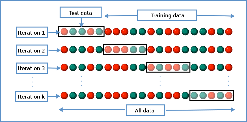
Each subset used once as the held-out set, and \(K - 1\) times for training
Cross-validation cartoon
Gives \(K\) estimates of the held-out error at each \(\lambda\). Credit: Wikipedia
\(K\)-fold cross-validation
Each subset used once as the held-out set, and \(K - 1\) times for training
Choose \(\hat\lambda\) to minimize \[
\hat R_{K\text{-cv}}(\lambda) = \frac1K\sum_{k=1}^K \hat R_k\big(\hat f^{(k)}_\lambda\big)
\] where \(\hat f^{(k)}_\lambda\) is fitted on the data that “holds out” the \(k\)th fold, and \(\hat R_k\) is its error on that fold
Then refit the model \(\hat f_{\hat\lambda}\) at that value \(\hat\lambda\) on the entire dataset
The CV curve on the Spotify tracks
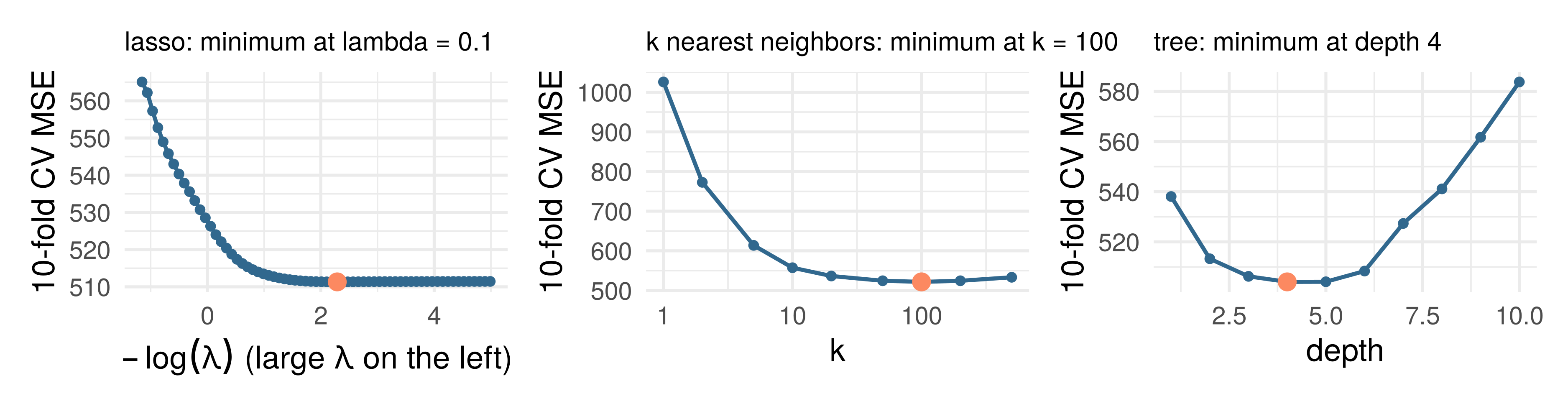
The 5,000 training tracks, \(K = 10\). One curve per family, the knob where each is lowest (orange). Every fold’s fit standardizes on its own training rows. The selection set was not used: each track was fitted on nine times and scored once
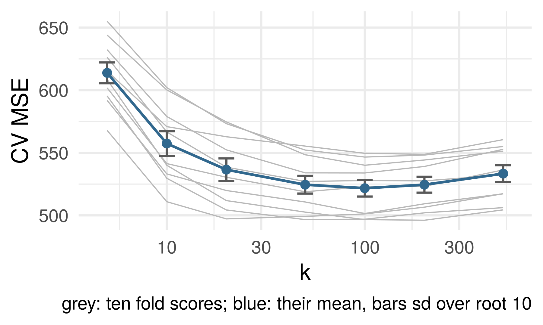
Standard errors: held out, and the CV bars
A flat bottom: \(k = 50\) to \(200\) are within one bar of each other
A held-out score is a mean of \(m\) losses \(L_j = \ell(y_j, \hat f(x_j))\), independent with \(\hat f\) fixed: \[
\widehat{\text{Err}} = \frac1m\sum_{j=1}^m L_j, \qquad \text{SE} = \frac{\text{sd}(L)}{\sqrt m}
\] The structures lecture’s bars: \(m = 2{,}000\) selection tracks. Software’s CV bars: the same formula on the \(K\) fold scores, \(m = K\); a heuristic, since the folds share fitting rows
Lessons about cross-validation
Think of it as a way to choose model complexity, not the model itself
Beware common cross-validation errors! From Duda and Hart quoted in MLstory
… the same data were often used for designing and testing the classifier. This mistake is frequently referred to as “testing on the training data.” A related but less obvious problem arises when a classifier undergoes a long series of refinements guided by the results of repeated testing on the same data. This form of “training on the testing data” often escapes attention until new test samples are obtained.
Lessons about cross-validation
Beware common cross-validation errors! From ESL:
Ideally, the test set should be kept in a “vault,” and be brought out only at the end of the data analysis. Suppose instead that we use the test-set repeatedly, choosing the model with smallest test-set error. Then the test set error of the final chosen model will underestimate the true test error, sometimes substantially.
Cross-validate the entire model-building pipeline (not just one step), and only do it once – or at least not many times
Choosing \(K\): larger \(\to\)\(\hat R_{K\text{-cv}}\) has lower bias, more variance. Often use \(K = 5\) or \(10\)
plot(cv.glmnet)
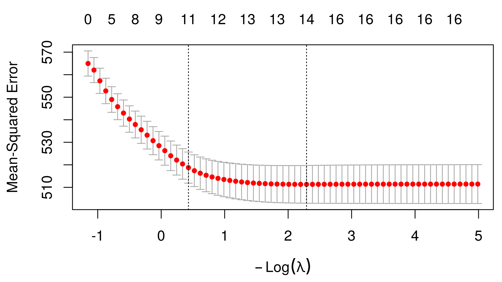
glmnet’s own cross-validation of the lasso on the training tracks, the same ten folds. Top axis: how many coefficients are nonzero
cv_fit <-cv.glmnet(X, y, foldid = fold)plot(cv_fit)
Dotted lines: lambda.min, the minimum; lambda.1se, the largest \(\lambda\) within one bar of it, the one-standard-error rule
The bars, \(\text{sd}/\sqrt K\) of the fold scores, are a heuristic (the folds share rows). The minimum is chosen among 67 candidates on these rows: biased low, a score to choose with, not to report
Part 2: the nearest-neighbor rate
Why care about rates?
Over a trillion dollars is going into scaling up AI models. What if this is mathematically guaranteed to fail?
The CV curve put \(k\) at 100 on 5,000 tracks and \(p = 11\) inputs. Where would the minimum be with 50,000 tracks? With 110 inputs?
Bias–variance decomposition, \(k\)-NN form: inputs fixed, \(y_i = f^\star(x_i) + \varepsilon_i\), \(\varepsilon_i\) independent, mean \(0\), variance \(\sigma^2\); \(\hat f_k(x_0)\) the mean of the \(k\) nearest \(y_i\): \[
\mathbb E\big[(Y_0 - \hat f_k(x_0))^2\big] = \sigma^2 + \Big[f^\star(x_0) - \tfrac1k\textstyle\sum_l f^\star(x_{(l)})\Big]^2 + \sigma^2/k
\]
The variance term is explicit, \(\sigma^2/k\). The bias term depends on \(f^\star\) at the \(k\) nearest inputs, and can be bounded only by an assumption on \(f^\star\)
What assumption on \(f^\star\) makes the bias term a number? Write it down.
\(k\)-NN rate: bounding the bias
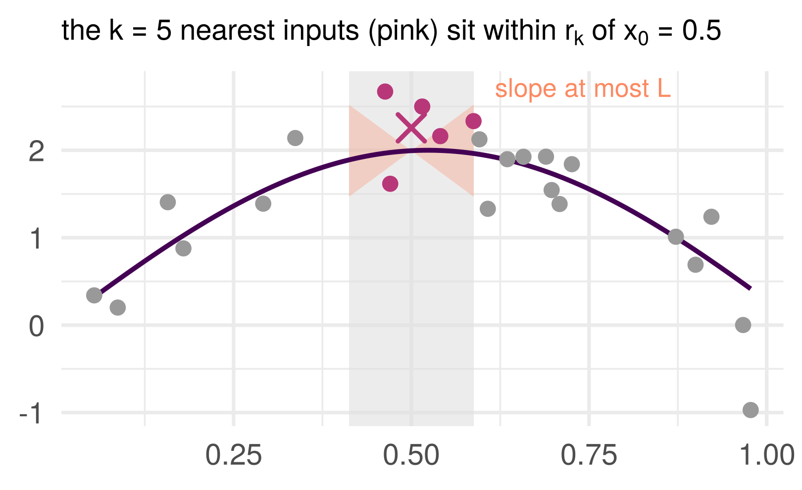
\(r_k(x_0)\): the distance from \(x_0\) to its \(k\)th nearest training input. Every neighbor is within it
Assume\(f^\star\) is \(L\)-Lipschitz: \(|f^\star(x) - f^\star(x')| \le L\,\|x - x'\|\). Then each neighbor’s \(f^\star\) is within \(L\,r_k\) of \(f^\star(x_0)\), so their average is too
Proof. “Inputs fixed”: given the training inputs \(x_1, \ldots, x_n\), the neighbors are fixed and only the noise is random. The bias \(\frac1k\sum_l [f^\star(x_{(l)}) - f^\star(x_0)]\) has each term at most \(L\,r_k\) in size, so its square is at most \(L^2 r_k^2\); the variance is \(\sigma^2/k\). \(\blacksquare\)
The nearest-neighbor distance lemma
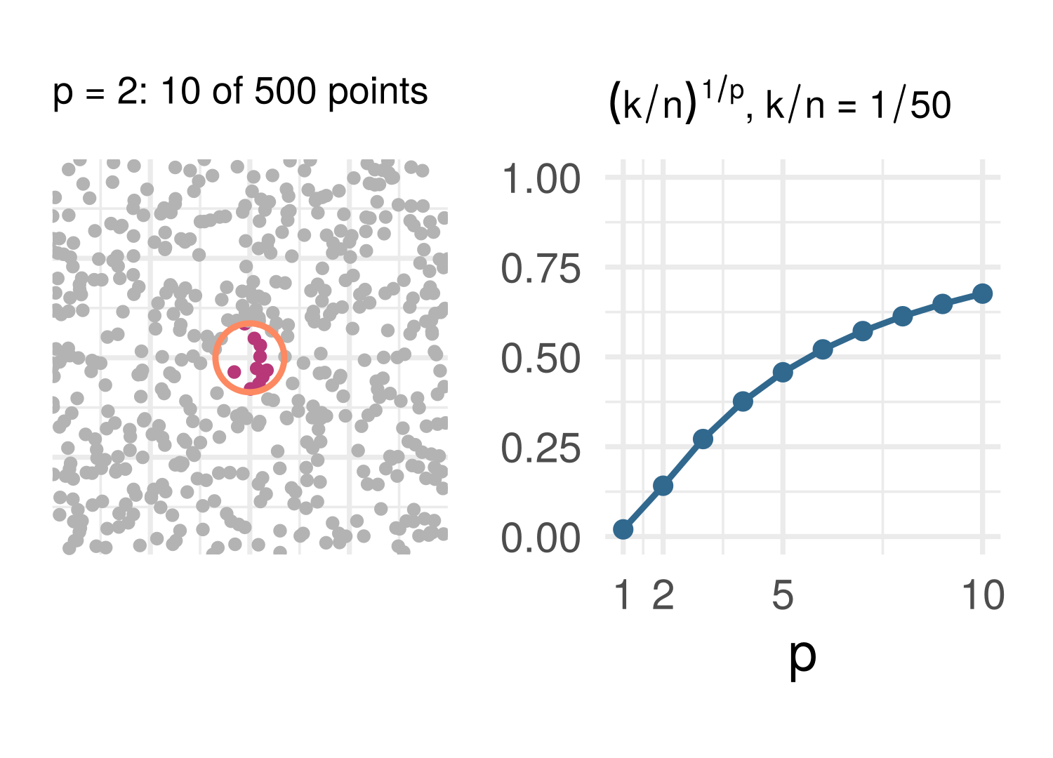
How far away is the \(k\)th neighbor? Inputs i.i.d. uniform on \([0, 1]^p\). A ball around \(x_0\) holding \(k\) of the \(n\) points has volume about \(k/n\), so its radius is about \((k/n)^{1/p}\)
Nearest-neighbor distance lemma (stated). For \(x_0\) away from the boundary, \(\mathbb E\big[r_k(x_0)^2\big] \le C_p\,(k/n)^{2/p}\), with \(C_p\) depending on \(p\) only.
In one dimension the \(k\)th neighbor is about \(k/2n\) away on each side. In \(p = 10\) the radius is about \((k/n)^{1/10}\): with \(k/n = 1/100\), \(0.63\) of the side of the cube
Curse of dimensionality: in many dimensions, the nearest \(1\%\) of the data is not near.
The rate
Put the two together and choose \(k\): \[
\mathbb E\big[(\hat f_k(x_0) - f^\star(x_0))^2\big] \;\le\; C_p L^2 (k/n)^{2/p} + \sigma^2/k
\] The first term grows with \(k\), the second shrinks. They balance at \(k = c\,n^{2/(p+2)}\), and there \[
\text{error} \le C\, n^{-2/(p+2)}, \qquad c, C \text{ constants not depending on } n
\]
To halve the bound, \(2^{(p+2)/2}\) times the data: \(2.8\times\) in \(p = 1\), \(4\times\) in \(p = 2\), \(64\times\) in \(p = 10\)
Minimax rate (stated). Over all \(L\)-Lipschitz \(f^\star\) in \(p\) dimensions no estimator beats \(n^{-2/(p+2)}\) for every \(f^\star\) (Stone 1980, 1982); a particular \(f^\star\), a constant say, does better.
The cost of a non-free lunch
Assumption on \(f^\star\)
Squared error (up to constants; rows 1 and 2 minimax)
The family
\(L\)-Lipschitz in \(p\) inputs
\(n^{-2/(p+2)}\)
nearest neighbors, a tree, a network: smoothness only
a sum of a fixed number of Lipschitz one-input curves (additivity, plus design conditions)
\(n^{-2/3}\), the one-input rate (Stone 1985)
additive splines: no interactions
linear with \(s\) nonzero coefficients among \(p\) (sparsity, plus design and noise conditions)
about \(s\log p/n\), an upper bound (Hastie et al. 2015, Theorem 11.2)
the lasso: a sparse plane
Smoothness alone: \(p\) in the exponent. Additivity: the one-input exponent. Sparsity: \(p\) out of the exponent, into a \(\log p\). Rows 2 and 3 are stated, not derived
No free lunch theorem, with numbers. A faster rate needs a stronger assumption.
Part 3: ridge and the lasso side by side
Assumptions \(\leftrightarrow\) biases?
History: Stein’s paradox
Estimating \(\mu \in \mathbb R^p\) from an i.i.d. sample \(\mathbf Y_1, \ldots, \mathbf Y_n \sim N(\mu, \sigma^2 I)\). The MLE is \(\bar{\mathbf Y}\) (obvious and best, right?)
The James–Stein estimatorshrinks\(\bar{\mathbf Y}\) toward some other point, any other point, chosen a priori, e.g. 0: \[
\hat\mu_{\text{JS}} = \Big(1 - \frac{(p-2)\sigma^2/n}{\|\bar{\mathbf Y}\|^2}\Big)\bar{\mathbf Y}, \qquad \text{MSE}(\hat\mu_{\text{JS}}) < \text{MSE}(\bar{\mathbf Y}) \text{ for all } \mu, \text{ if } p > 2
\]
Ridge’s estimates are dense: every coefficient nonzero, in general; the lasso’s are exactly zero over whole ranges of \(\lambda\). What \(\lambda\) does to one coefficient is hidden in general, because the coefficients interact; in the simplest design they do not
The identity design
\(\mathbf X = I\) (\(n = p\)), so \(\mathbf y = \beta + \boldsymbol\varepsilon\): one observation per coefficient, least squares \(\hat\beta = \mathbf y\). A penalty that adds up over coefficients, as ridge’s and the lasso’s do, splits the objective: \(\|\mathbf y - \beta\|_2^2 + \mathcal P_\lambda(\beta) = \sum_j \big[(y_j - \beta_j)^2 + \mathcal P_\lambda(\beta_j)\big]\), one problem per coefficient
Ridge: \(\hat\beta_{\lambda, j} = \dfrac{y_j}{1 + \lambda}\), every coefficient shrunk by the same factor, zero only if \(y_j = 0\)
Lasso: \(\hat\beta_{\lambda, j} = \mathrm{sign}(y_j)\,\big(|y_j| - \tfrac{\lambda}{2}\big)_+\), each \(y_j\) moved toward zero by \(\lambda/2\), stopping at zero: exactly zero whenever \(|y_j| \le \lambda/2\)
Soft thresholding.\(\arg\min_b\ (y - b)^2 + \lambda|b| = \mathrm{sign}(y)\,(|y| - \lambda/2)_+\). Deriving both minimizers: an exercise in the notebook.
Bias–variance decomposition, ridge form
Same design, noise variance \(\sigma^2\). Least squares, \(\hat\beta = \mathbf y\): unbiased, variance \(\sigma^2\) per coefficient. Divide by \(1 + \lambda\): \[
\text{bias}_j = -\frac{\lambda}{1 + \lambda}\,\beta_j, \qquad \mathrm{Var}(\hat\beta_{\lambda,j}) = \frac{\sigma^2}{(1 + \lambda)^2}
\]
Bias–variance decomposition, ridge form.\(\mathbf X = I\), \(\mathbf y = \beta + \boldsymbol\varepsilon\), noise independent, mean \(0\), variance \(\sigma^2 > 0\): \(\;\mathrm{MSE}(\lambda) = \mathbb E\|\hat\beta_\lambda - \beta\|^2 = \sum_{j=1}^p (\lambda^2\beta_j^2 + \sigma^2)/(1 + \lambda)^2\), with slope \(-2p\sigma^2 < 0\) at \(\lambda = 0\): for every \(\beta\), some \(\lambda > 0\) beats least squares.
Proof: an exercise in the notebook. Which \(\lambda\)? The best is \(\sigma^2\) over the mean of \(\beta_j^2\), noise over signal: unknown
High-dimensional example
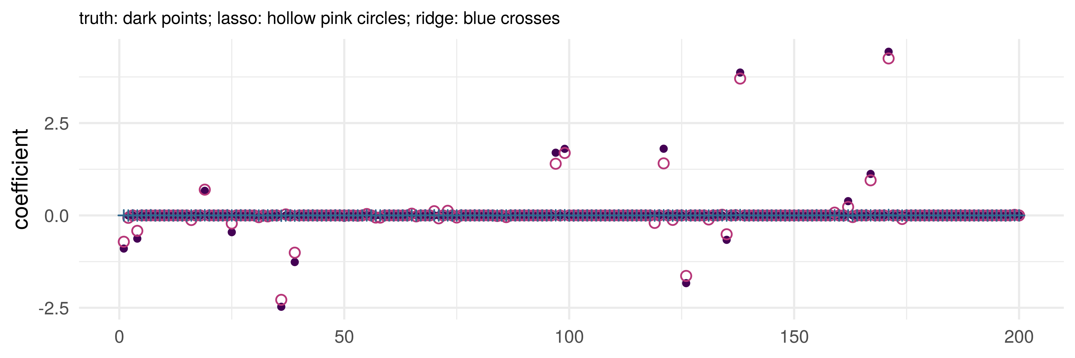
\(n = 100\) observations, \(p = 200\) inputs, \(\mathbf y = \mathbf X\beta + \boldsymbol\varepsilon\) with only 16 nonzero coefficients. Lasso and ridge at the \(\lambda\) cross-validation chooses
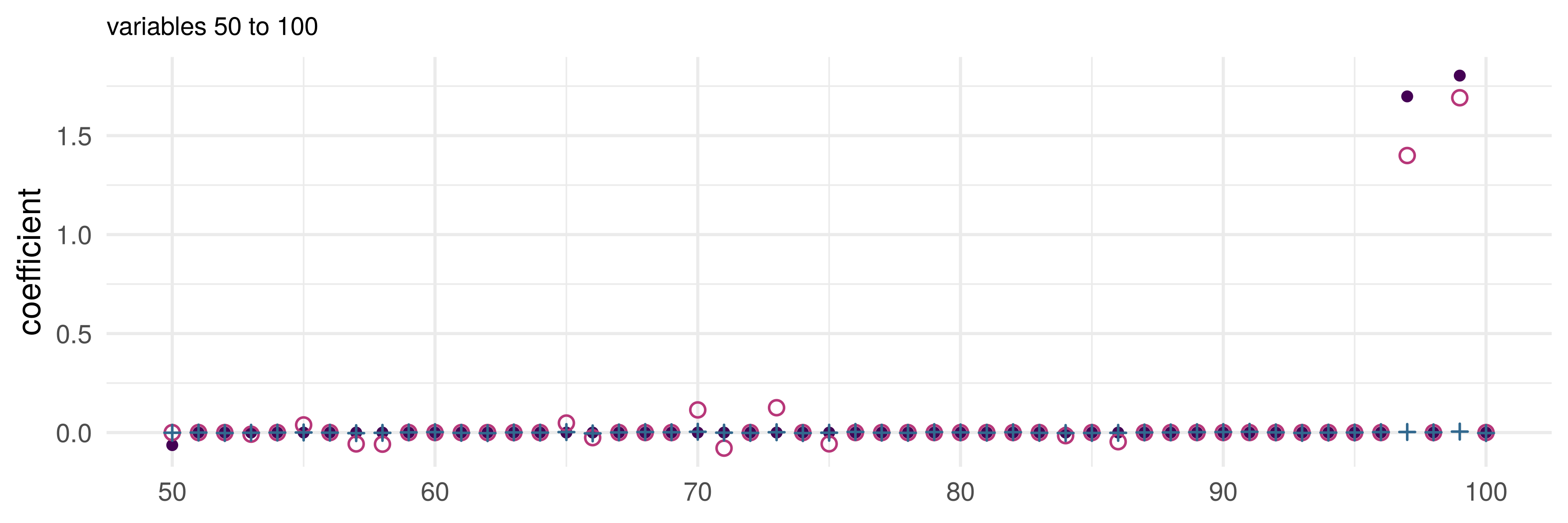
Zoom in on variables 50 to 100
Lasso: cool or extremely cool?
Penalized regression biases coefficients toward zero
The lasso usually sets some of them all the way to zero, so it does variable selection as it fits
People like sparser, simpler models: they can be easier to interpret
Lasso downside: instability
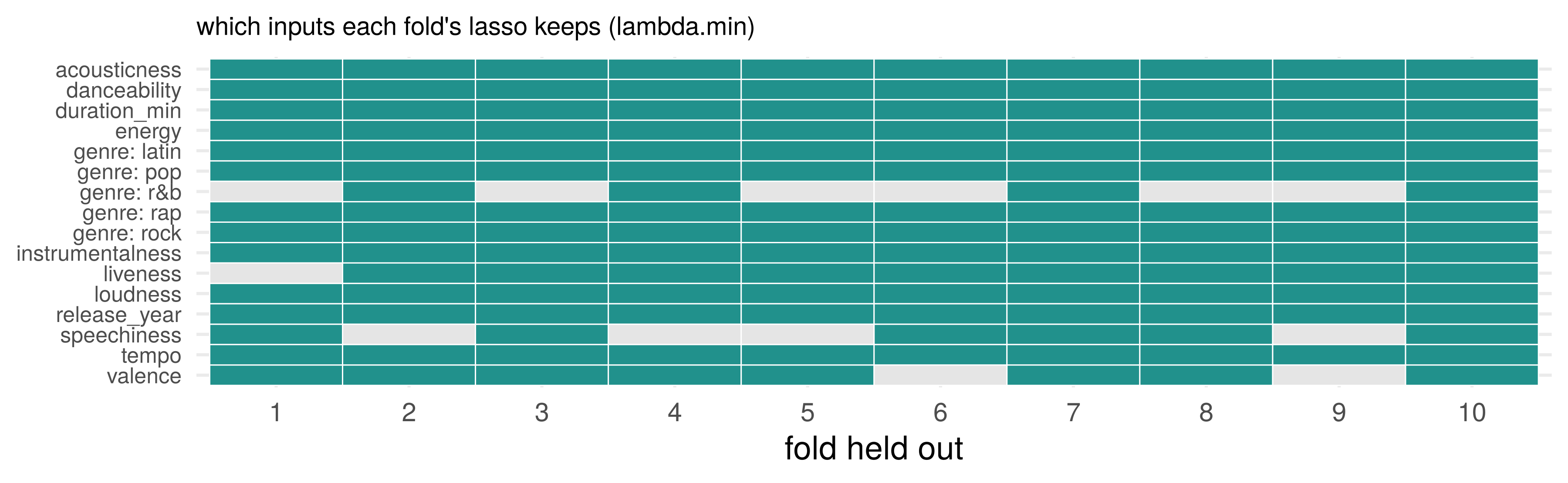
The ten models cross-validation fit, each on nine folds, at lambda.min: the kept inputs change from fold to fold. The same instability as a tree’s cutoffs. At the one-SE \(\lambda\) the ten sets agree
A fixed \(\lambda\) and a data-chosen \(\hat\lambda\)
\(\hat\beta_{\text{lasso}}(\lambda)\) at a fixed \(\lambda\)
\(\hat\beta_{\text{lasso}}(\hat\lambda)\) at a data-chosen \(\hat\lambda\)
Different in general! Theoretical results about the first (the rate, the ridge-form decomposition at a fixed \(\lambda\)) may not apply to the second
Choosing on a dataset is empirical risk minimization over a finite class: the winner’s score on the rows it was chosen on is biased low.
Part 4: a penalty on wiggliness
A penalty on wiggliness
The spline of the structures lecture: \(f(x) = \beta_0 + \sum_{j=1}^J \beta_j b_j(x)\), \(J\) the knob. Instead: take a large \(J\) as a ceiling, and penalize wiggliness
\[
\min_f\; \textstyle\sum_{i=1}^n \big(y_i - f(x_i)\big)^2 + \lambda\int f''(x)^2\,dx
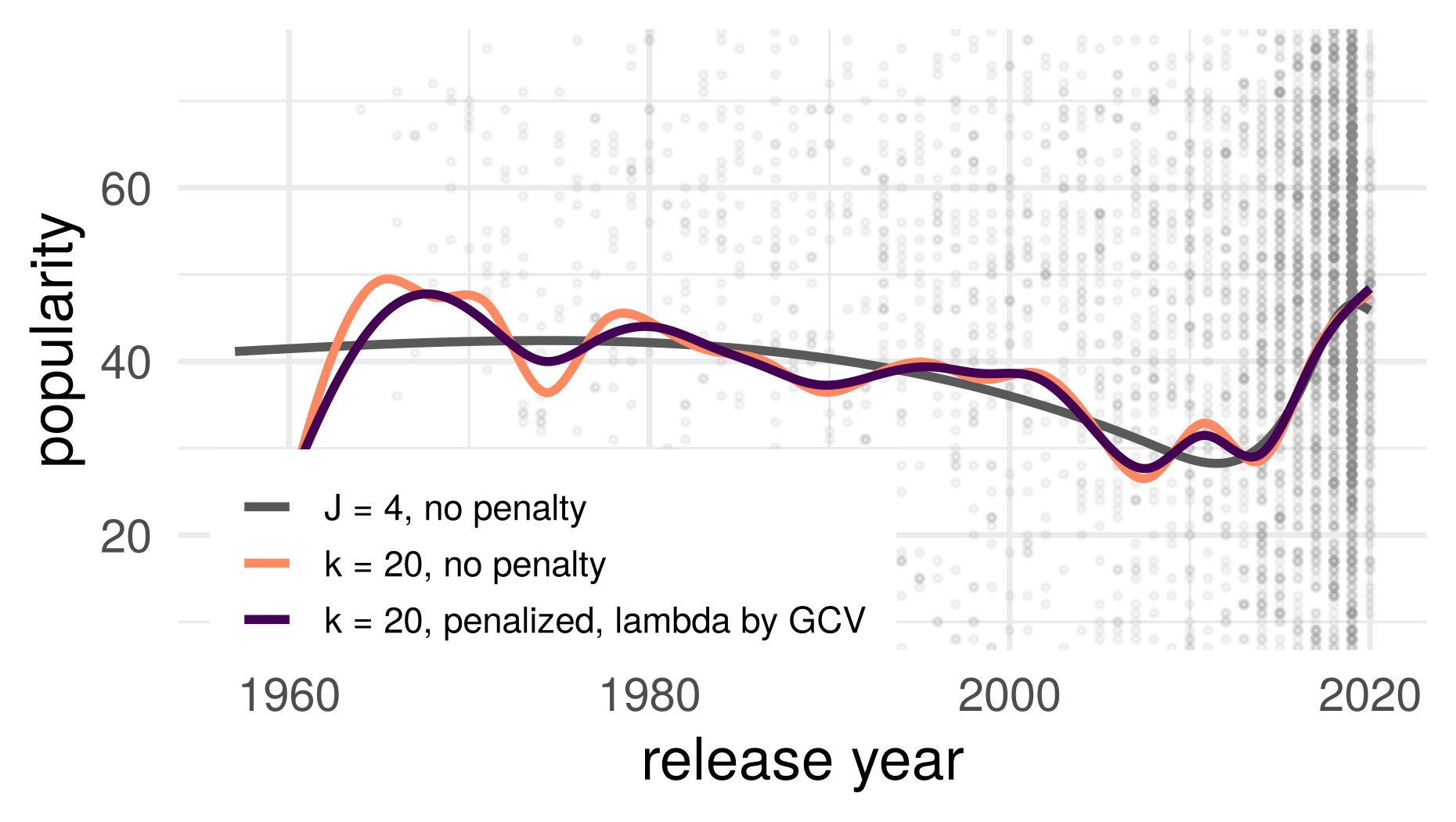
\]\(\lambda = 0\): the \(J\)-basis fit. \(\lambda \to \infty\): \(f'' = 0\), a straight line. In between: \(\lambda\) chosen by generalized cross-validation (GCV, mgcv’s default)
library(mgcv)gam(track_popularity ~s(release_year, k =20, bs ="cr"), data = sp_train)
The smoothing penalty as weighted ridge
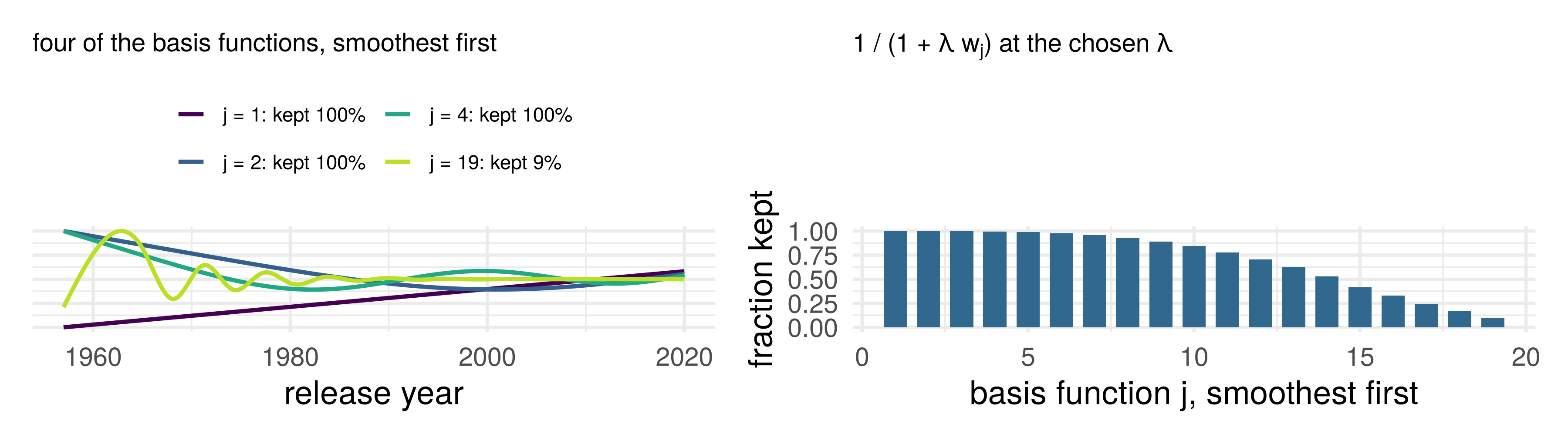
In the right basis, coefficient \(j\) is shrunk by \(1/(1 + \lambda w_j)\), \(w_j\) the wiggliness of basis function \(j\). The straight line (\(w = 0\)) is never shrunk; the wiggles nearly vanish. Ridge’s formula, with a weight
Part 5: double descent
The zero-error fits
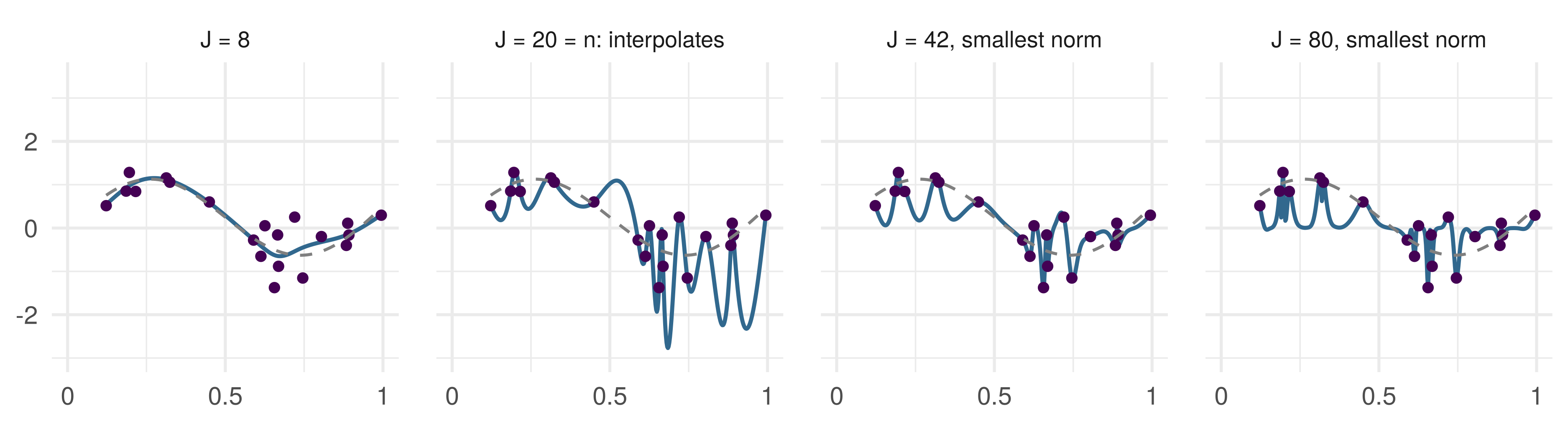
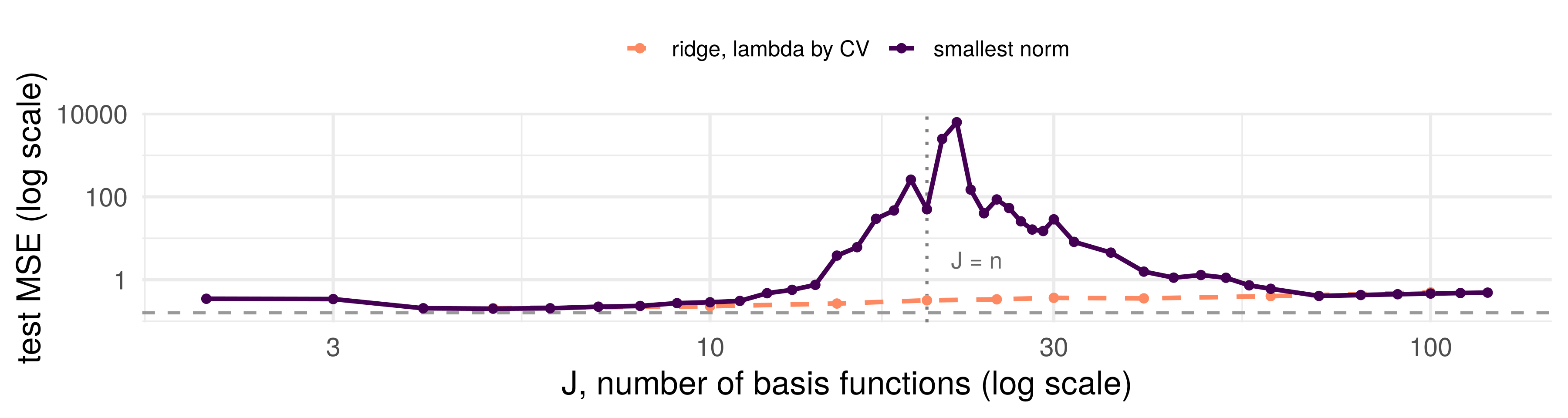
\(n = 20\) points, natural splines with \(J\) basis functions: least squares up to \(J = n\); beyond, of the many fits with zero training error, the one with the smallest \(\|\beta\|\) (ridge’s limit as \(\lambda \to 0\)). Zero training error does not say which fit you have: the rule that picks one is the regularization
Double descent, demonstrated
Test MSE against \(J\), averaged over 50 draws of 20 points: a U up to \(J = n\), a spike at \(J = n\) (interpolation threshold), a second descent beyond it (Belkin, Hsu, Ma and Mandal 2019). Ridge on same basis, \(\lambda\) by cross-validation: never interpolates, no spike. Dashed: noise variance
Does statistics apply to deep learning?
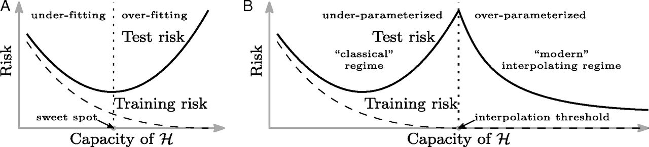
The bias–variance trade-off is one of the most important pillars of statistical wisdom. If we make a model too complex, it overfits to the training data… or does it?
Belkin, Hsu, Ma and Mandal (2019). Does zero training error necessarily mean the model is overfit? No. Anna Karenina principle: all truly optimal models are alike; each overfit model is overfit in its own way
Double descent: takeaways
It can happen for some models (large neural networks) on some data (high signal-to-noise: images, translation). So zero training error does not necessarily mean overfit, and a test error that has started rising might fall again later: we don’t know
It does not contradict the bias–variance trade-off. The decomposition holds at every point of both curves. The horizontal axis needs care: past \(J = n\), more basis functions is not more flexibility, so the curve need not be a U
For most methods in this course, expect a U: \(k\)-NN, trees, ridge, the lasso. Regularized fits do not interpolate, and have no second descent (the ridge curve)
ISLR section 10.8, pp. 441–443
Before the seminar
This week: exercises 1 and 2 at the top of the notebook. The ridge form of the bias–variance decomposition, proved in the orthogonal design with numbered hints; and the \(k\)-NN rate again, with the slides closed
In the seminar: a cross-validation pipeline on the Spotify tracks, written as one function and run for \(k\)-NN and the lasso; a learning-curve figure to read against the rate; and then, after it has worked, two ways cross-validation goes wrong
Conclusion
Cross-validation chooses the knob
Every row fitted on and scored on, in turn. The curve’s minimum is a chosen number: report a score from the vault
The error of a smooth \(f^\star\), in \(n\) and \(p\)
The worst-case rate is \(n^{-2/(p+2)}\) with smoothness alone; a stronger assumption gives a faster rate, when it holds
Ridge divides, the lasso subtracts
Bias on purpose: for every \(\beta\) some \(\lambda > 0\) beats least squares; the lasso’s zeros are exact. A penalty on wiggliness is ridge with weights. Past \(p = n\), the rule that picks the fit is the regularizer
References
Belkin, M., Hsu, D., Ma, S. and Mandal, S. (2019). Reconciling modern machine-learning practice and the classical bias–variance trade-off. Proceedings of the National Academy of Sciences 116(32), 15849–15854. doi:10.1073/pnas.1903070116
Hastie, T., Tibshirani, R. and Friedman, J. (2009). The Elements of Statistical Learning: Data Mining, Inference, and Prediction, 2nd edition. Springer, New York. Section 7.2, p. 222 (the quotation). hastie.su.domains/ElemStatLearn
Hastie, T., Tibshirani, R. and Wainwright, M. (2015). Statistical Learning with Sparsity: The Lasso and Generalizations. Chapman and Hall/CRC. Theorem 11.2(b), equation (11.26b), p. 300 (prediction error); Theorem 11.1 and Example 11.1, pp. 295–296 (coefficient error). doi:10.1201/b18401; free PDF at hastie.su.domains/StatLearnSparsity
References, continued
James, G., Witten, D., Hastie, T. and Tibshirani, R. (2021). An Introduction to Statistical Learning with Applications in R, 2nd edition. Springer, New York. Section 10.8 and Figure 10.21, pp. 439–443 (the zero-error fits, adapted). statlearning.com
Stone, C. J. (1980). Optimal rates of convergence for nonparametric estimators. Annals of Statistics 8(6), 1348–1360. doi:10.1214/aos/1176345206
Stone, C. J. (1982). Optimal global rates of convergence for nonparametric regression. Annals of Statistics 10(4), 1040–1053. doi:10.1214/aos/1176345969
Stone, C. J. (1985). Additive regression and other nonparametric models. Annals of Statistics 13(2), 689–705. doi:10.1214/aos/1176349548