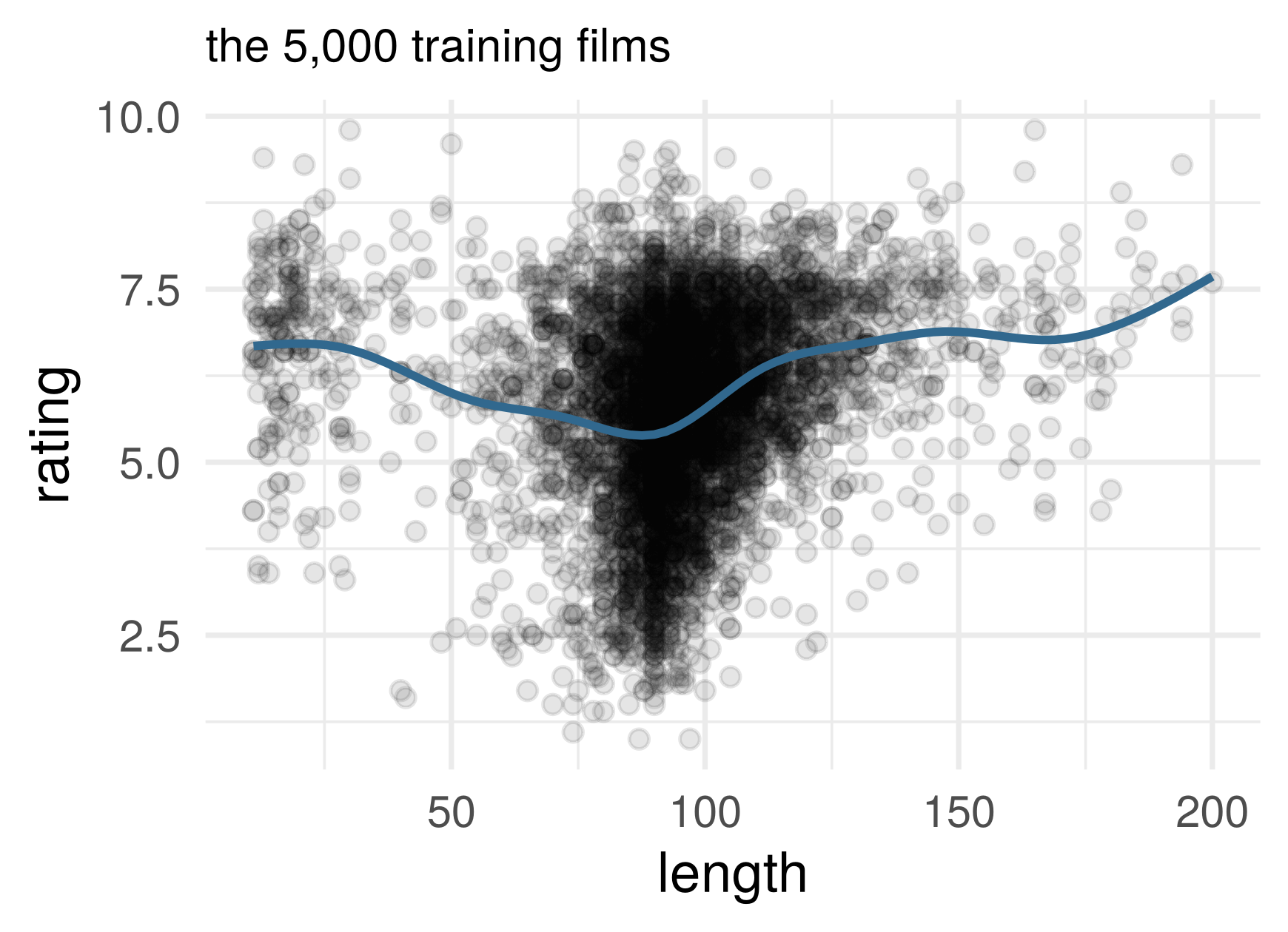
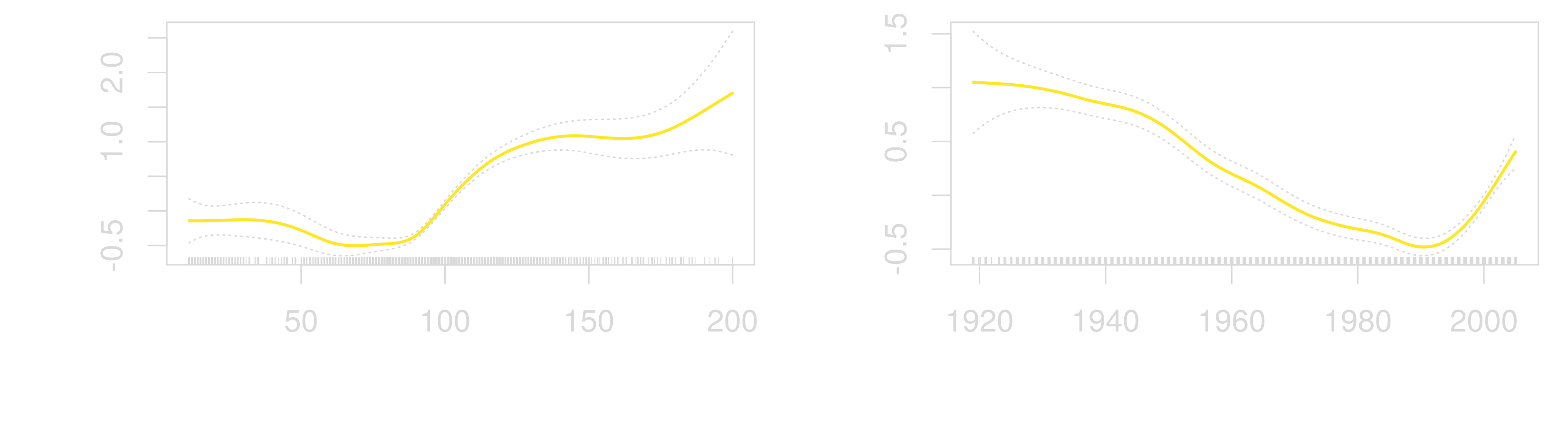
The cost of a non-free lunch: a sum of a fixed number of Lipschitz one-input curves (additivity, plus design conditions) has the one-input rate, \(n^{-2/3}\).
Fitting several curves
Could we fit this model one curve at a time?
Backfitting algorithm
Model: \(\hat f(x_1, \ldots, x_p) = \hat\beta_0 + \hat f_1(x_1) + \cdots + \hat f_p(x_p)\). Columns \(\mathbf x_1, \ldots, \mathbf x_p\); \(\hat f_k(\mathbf x_k)\) is the vector of fitted values of curve \(k\)
Initialize: \(\hat\beta_0 = \bar y\), and \(\hat f_j^{(0)} = 0\) for every \(j\)
\(\hat f_j^{(t)}\): a one-input smoother (e.g. a spline) of \(\mathbf r_j^{(t)}\) on \(\mathbf x_j\), centered to mean zero
stop when iteration \(t\) barely changes the fitted values
Backfitting and partialling out
Two centered inputs, and a line for each component: \(\hat f_j(x) = \hat\beta_j x\). Start at \(\hat\beta_2^{(0)} = 0\). Iteration \(t\) fits each slope to its partial residual: \[
\hat\beta_1^{(t)} = \frac{\mathbf x_1^T\big(\mathbf y - \hat\beta_2^{(t-1)} \mathbf x_2\big)}{\mathbf x_1^T \mathbf x_1}, \qquad
\hat\beta_2^{(t)} = \frac{\mathbf x_2^T\big(\mathbf y - \hat\beta_1^{(t)} \mathbf x_1\big)}{\mathbf x_2^T \mathbf x_2}
\]
The slopes stop changing only where both hold: \(\mathbf x_j^T(\mathbf y - \hat\beta_1 \mathbf x_1 - \hat\beta_2 \mathbf x_2) = 0\) for \(j = 1, 2\). These are the normal equations: the fixed point is least squares
Partialling-out theorem: the coefficient on \(\mathbf x_2\) is \(\tilde{\mathbf x}_2^T \mathbf y / \tilde{\mathbf x}_2^T \tilde{\mathbf x}_2\), the slope on what is left of \(\mathbf x_2\) after \(\mathbf x_1\) has explained what it can.
Backfitting does this with smooth curves instead of lines
Backfitting on the films
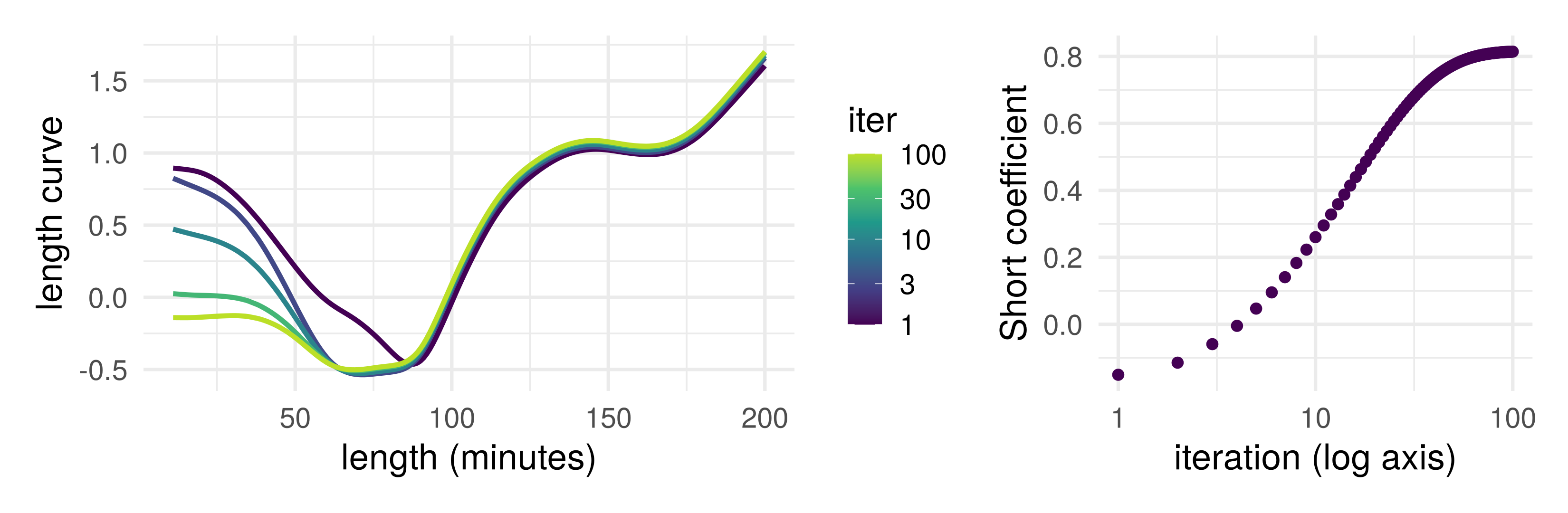
Length, year and Short on the training films, starting from zero. Length and Short are closely related: each iteration moves a little more of the shorts’ higher ratings from the length curve to the Short coefficient, which settles after about 70 iterations
Backfitting, more generally
Any number of inputs. With one coefficient per input, each update minimizes the RSS over that coefficient with the others held fixed: coordinate descent (Gauss–Seidel, in numerical linear algebra). A spline gives each input a block of coefficients, updated together: block coordinate descent. Fast for unrelated inputs, slow for strongly related ones
Gram–Schmidt residualizes each input (predictor) on the ones before it, once. Backfitting leaves the inputs alone and residualizes \(\mathbf y\) iteratively
Partialling out with flexible fits. Residualize both \(\mathbf y\) and \(\mathbf x_j\) on the other inputs, with any regression method, then regress residual on residual: double machine learning, later in the course
Part 2: additivity vs interactions
Partial dependence plots for a GAM
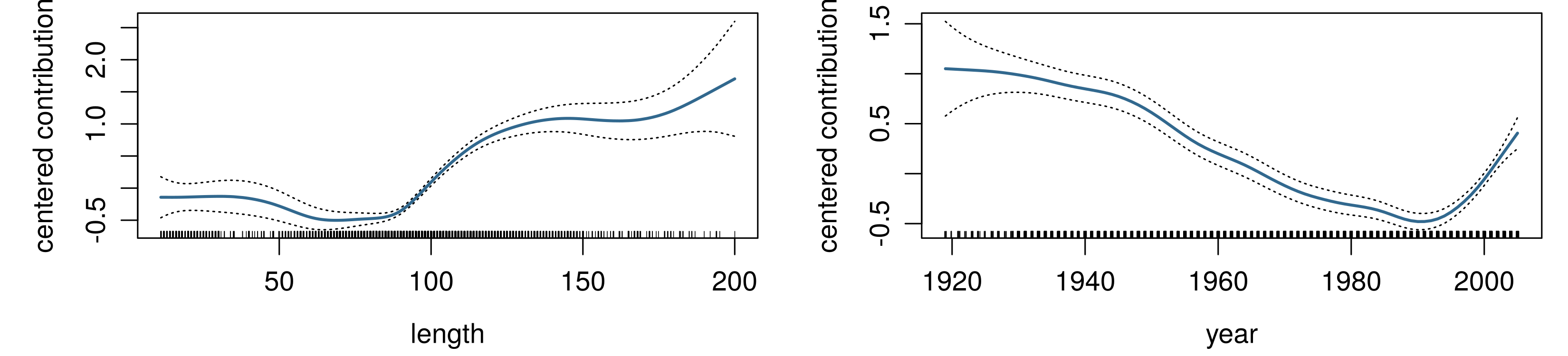
These univariate plots for GAMs are called partial dependence plots (PDPs), each up to a constant: for an additive fit, the partial dependence on \(x_j\) is \(\hat f_j\) plus a constant. They show how the GAM depends on each feature: a simple one-dimensional dependence, because of the additivity assumption
Since all models are wrong the scientist must be alert to what is importantly wrong. It is inappropriate to be concerned about mice when there are tigers abroad.
Box (1976), emphasis added
Remember that all models are wrong; the practical question is how wrong do they have to be to not be useful.
Box and Draper (1987)
Can additivity/GAMs be importantly wrong?
Interpretation: think carefully about calculus and causality (causality: briefly, after the interactions). To simplify let’s consider the identity link function (rather than e.g. logistic regression, those cases are more complicated)
Calculus
Does the CEF really decompose into additive terms? Is this approximation good:
\[
\frac{\partial}{\partial x_j} \mathbb E[Y | \mathbf X] \approx f_j'(x_j)
\] Or does the relationship between the average of \(Y\) and \(x_j\) vary depending on the value of another predictor \(x_k\)?
Interactions in the movies data
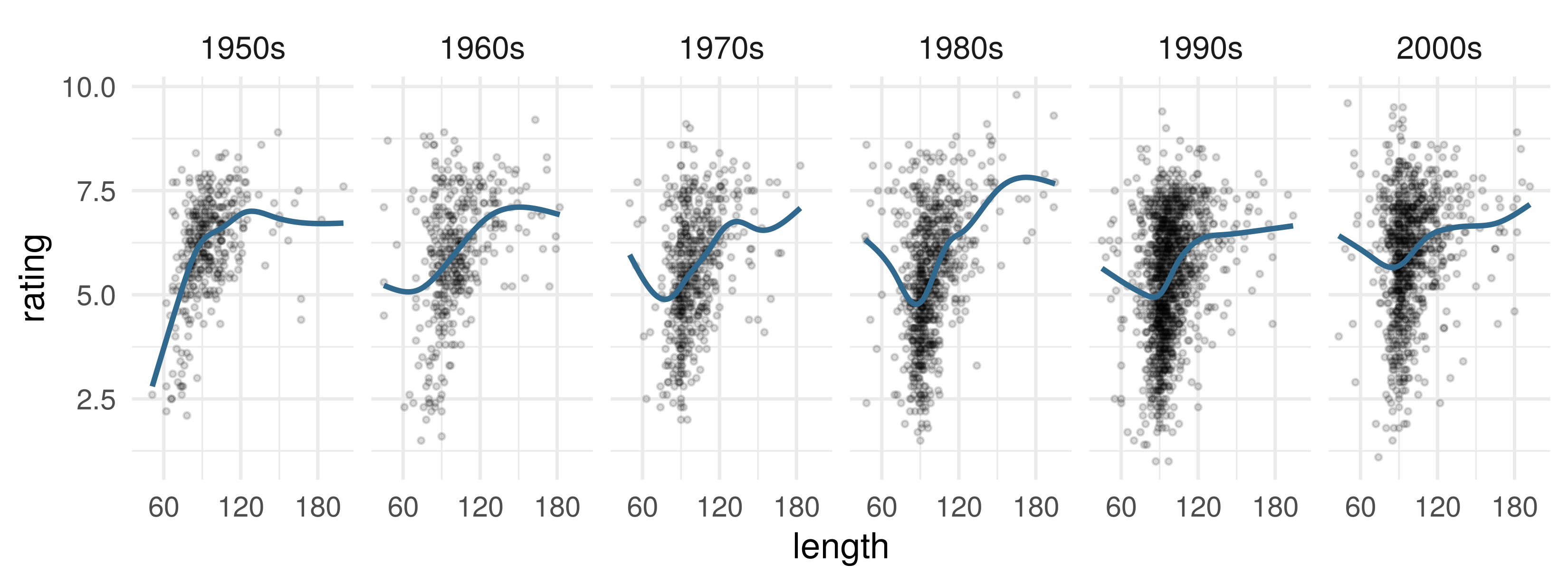
If the slope in length changes with year, the derivative of \(\mathbb E[\text{rating} \mid \text{length}, \text{year}]\) in length depends on year too, and an additive model is misspecified. Non-shorts, by decade:
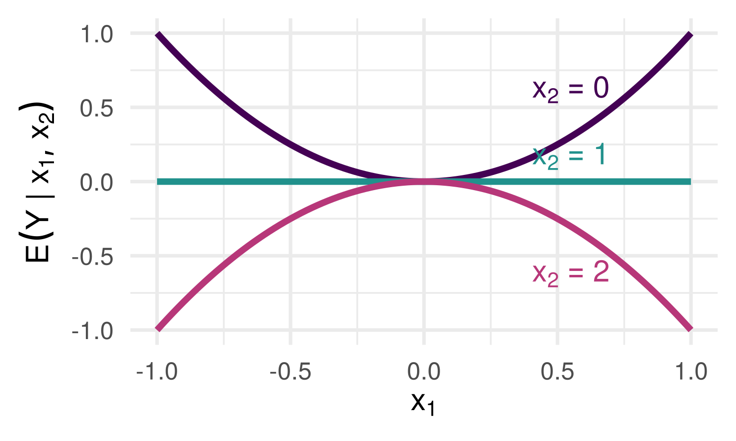
True model non-additive; GAM is wrong
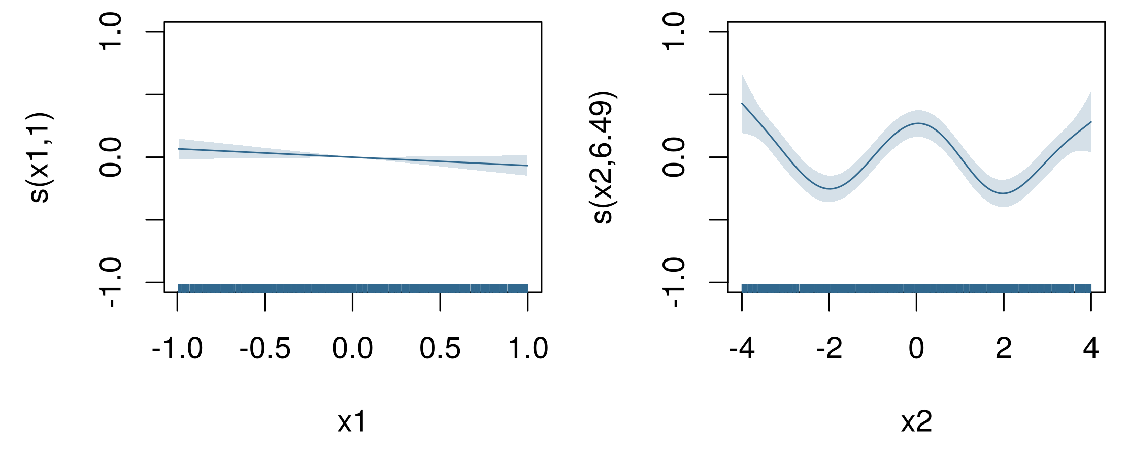
f1 <-function(x) x^2f2 <-function(x) cos(pi * x /2)df_int <-tibble(x1 =runif(2000, -1, 1), x2 =runif(2000, -4, 4)) |>mutate(y =f1(x1) *f2(x2) +rnorm(2000))fit_gam_wrong <-gam(y ~s(x1) +s(x2), data = df_int)
The fitted component for \(x_1\) is nearly flat: the parabolas cancel when averaged over \(x_2\). Additivity assumption is now (importantly) wrong
Causality: what are we “controlling for”?
Louisiana v. Callais, US Supreme Court, 29 April 2026, 6 to 3: evidence of racially polarized voting must come from “an analysis that controls for party affiliation”
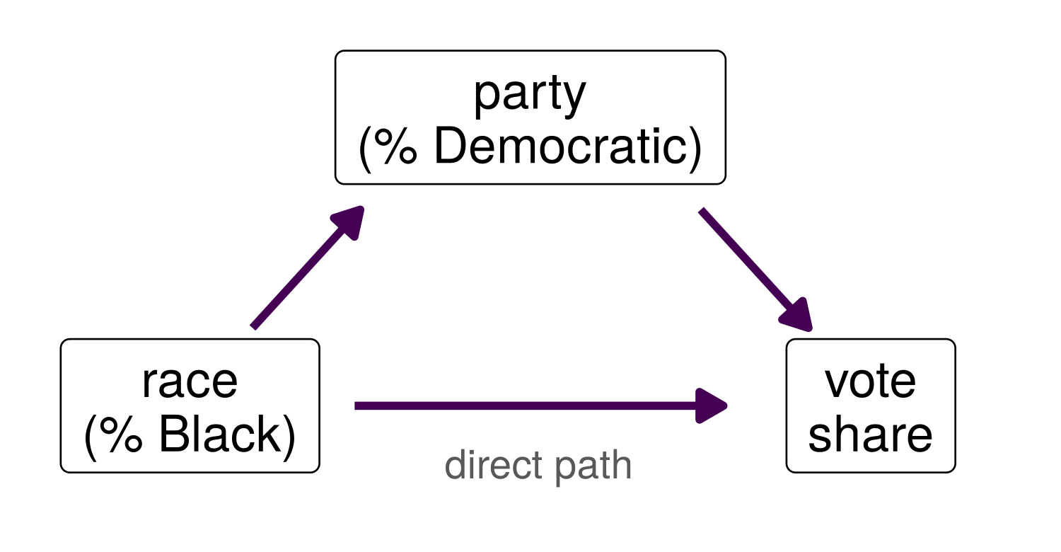
The majority’s reasoning: the divide may be partisan rather than racial, so race counts only where it survives holding party fixed
Critics argue that this misuses statistics: party is partly a consequence of race, so holding it fixed removes part of what is to be measured (Morris 2026)
After the decision, several Southern states redrew their congressional maps before the November 2026 midterm elections
What would a GAM of vote share on race and party show?
Causality: what partial dependence holds fixed
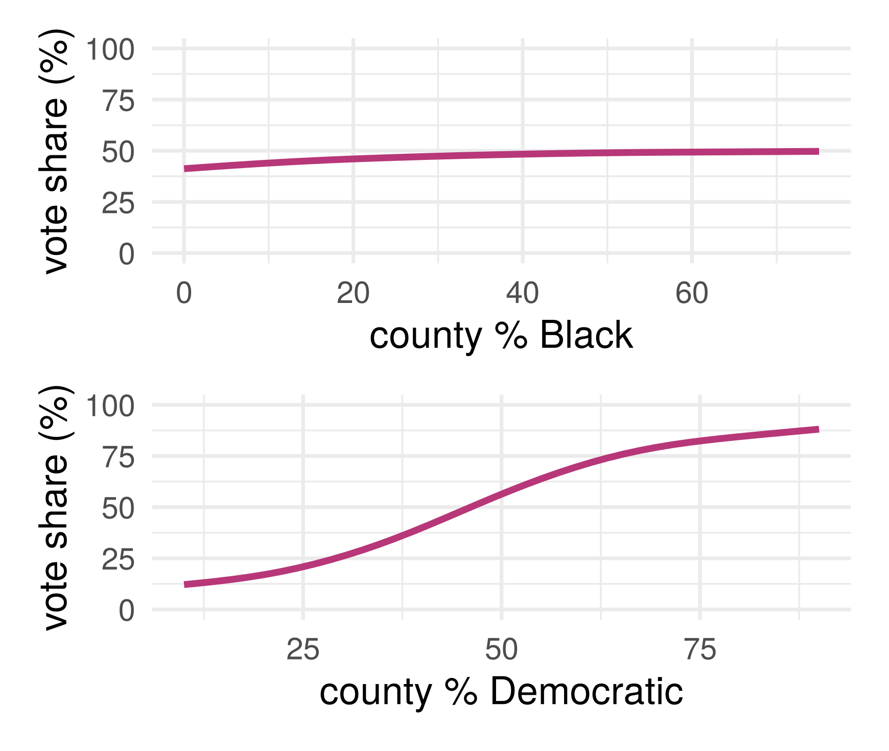
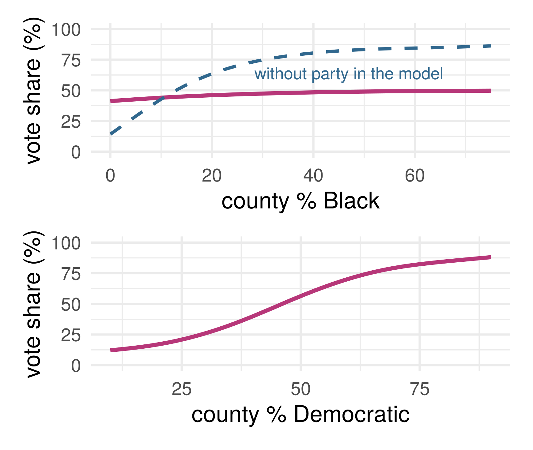
Simulated counties, an additive CEF, a GAM that fits it. Each partial dependence plot holds the other input fixed: the direct path only. Race acts mostly through party, a mediator
Recap: the causal example
The GAM fits correctly, the plot interprets the GAM correctly, but the plot answers the wrong (uninteresting) causal question
Adjustment theorem: adjust for common causes of \(T\) and \(Y\), and for no consequence of \(T\)
Part 3: building a tree
The Star Wars films
Episode
Film
Year
Length (minutes)
Rating
IV
Star Wars
1977
125
8.8
V
The Empire Strikes Back
1980
129
8.8
VI
Return of the Jedi
1983
135
8.1
I
The Phantom Menace
1999
133
6.4
II
Attack of the Clones
2002
120
7.0
Ratings: IMDb users’ averages, up to 2005
We’ll walk through growing and pruning a tree on this small subset of the data
RSS for each possible split
Split
Yes
No
Mean, yes
Mean, no
RSS
year < 1978.5
IV
V, VI, I, II
8.80
7.58
3.49
year < 1981.5
IV, V
VI, I, II
8.80
7.17
1.49
year < 1991
IV, V, VI
I, II
8.57
6.70
0.51
year < 2000.5
IV, V, VI, I
II
8.03
7.00
3.85
length < 122.5
II
IV, V, VI, I
7.00
8.03
3.85
length < 127
IV, II
V, VI, I
7.90
7.77
4.67
length < 131
IV, V, II
VI, I
8.20
7.25
3.61
length < 134
IV, V, I, II
VI
7.75
8.10
4.59
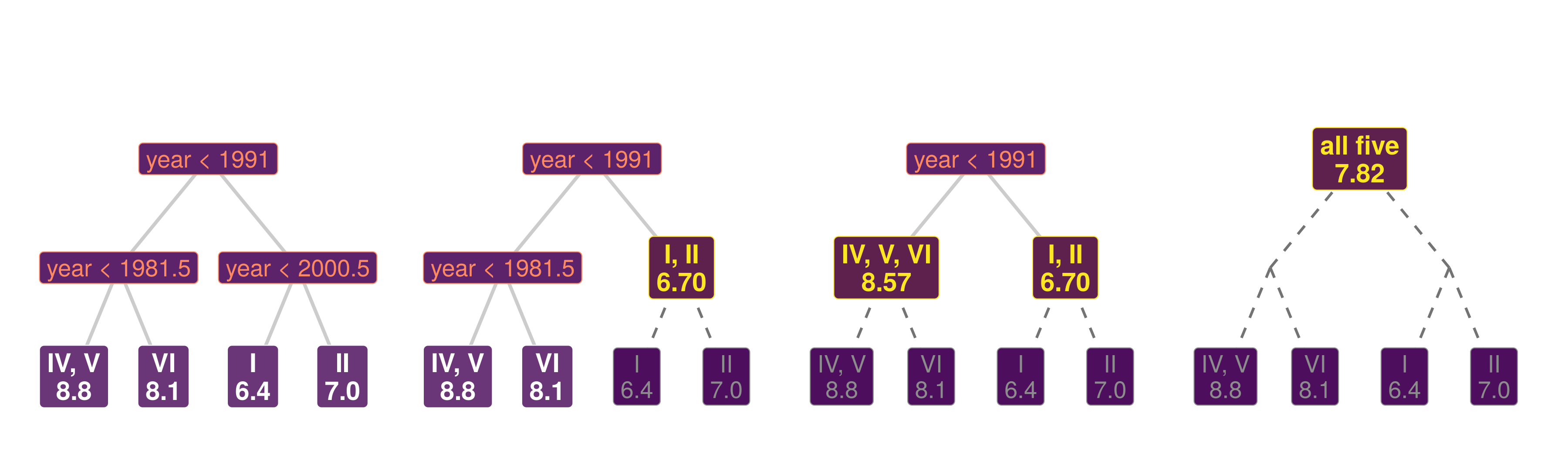
No split: every film predicted by the mean, 7.82, RSS 4.69. Each side of a split is a leaf; the search then recurses into each leaf
Recursion: RSS for each split inside each leaf
Yes to year < 1991: IV, V, VI (RSS 0.33)
Split
Yes
No
Mean, yes
Mean, no
RSS
year < 1978.5
IV
V, VI
8.80
8.45
0.25
year < 1981.5
IV, V
VI
8.80
8.10
0.00
length < 127
IV
V, VI
8.80
8.45
0.25
length < 132
IV, V
VI
8.80
8.10
0.00
No: I, II (RSS 0.18)
Split
Yes
No
Mean, yes
Mean, no
RSS
year < 2000.5
I
II
6.40
7.00
0.00
length < 126.5
II
I
7.00
6.40
0.00
Ties go to the first input, year. Every new leaf holds films of one rating: RSS 0, and growing stops
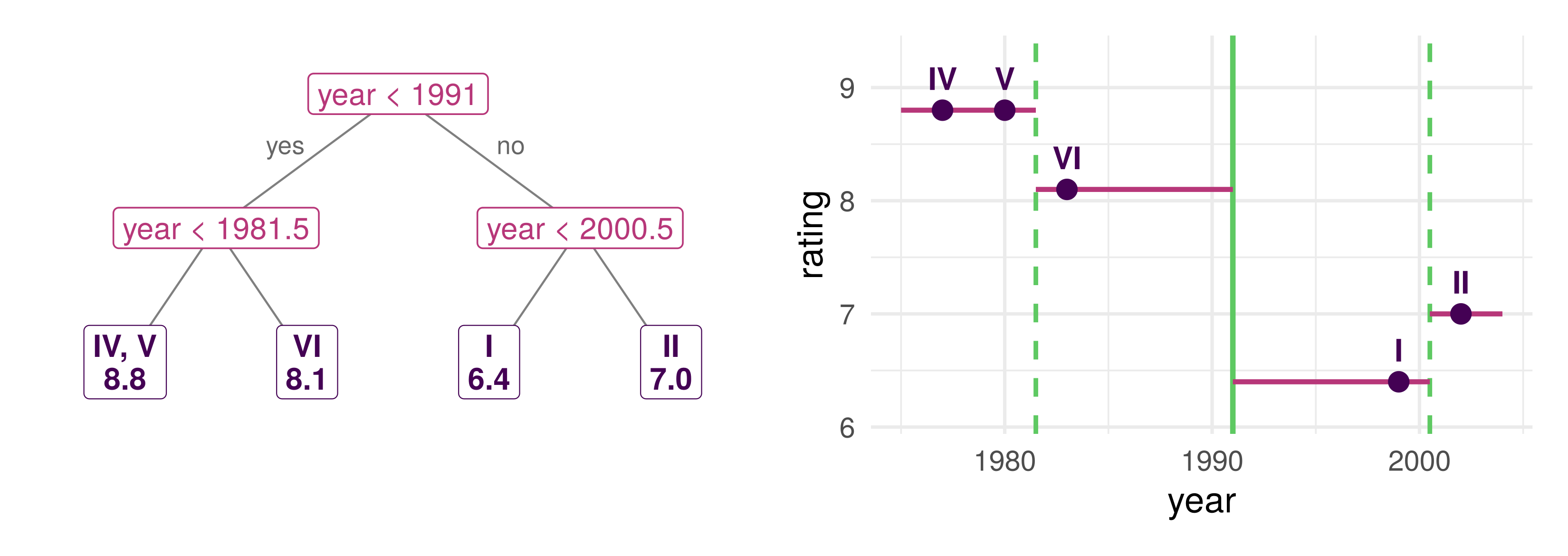
The grown tree
4 leaves, each holding films of one rating: a training RSS of 0. Grown until it cannot split, a tree memorizes its training data
Growing a tree
Recursive: split the data by the most discriminating single-variable question; then do the same inside each leaf, and so on
Greedy: each split is the best now. A weak split that would enable a strong one below it can be missed, so stopping early is risky: grow a large tree, then prune (next slide)
When to stop: a leaf too small to split (rpart’s minsplit), or no split that improves the fit enough (cp)
Grown until no leaf can split, a tree is like 1-nearest neighbors: on the training films, year and length alone give 2,670 leaves
\(k\) nearest neighbors average the \(k\) training points closest to \(x_0\); a tree averages those in \(x_0\)’s leaf, a neighborhood chosen by subsets of features
Pruning
For each \(\alpha \geq 0\), the sub-tree minimizing \(\text{RSS} + \alpha \times (\text{number of leaves})\). The Star Wars tree, as \(\alpha\) increases from 0:
Sequence of trees; tuning knob \(\alpha\) chosen by cross-validation or held-out data
Choosing \(\alpha\) on the films
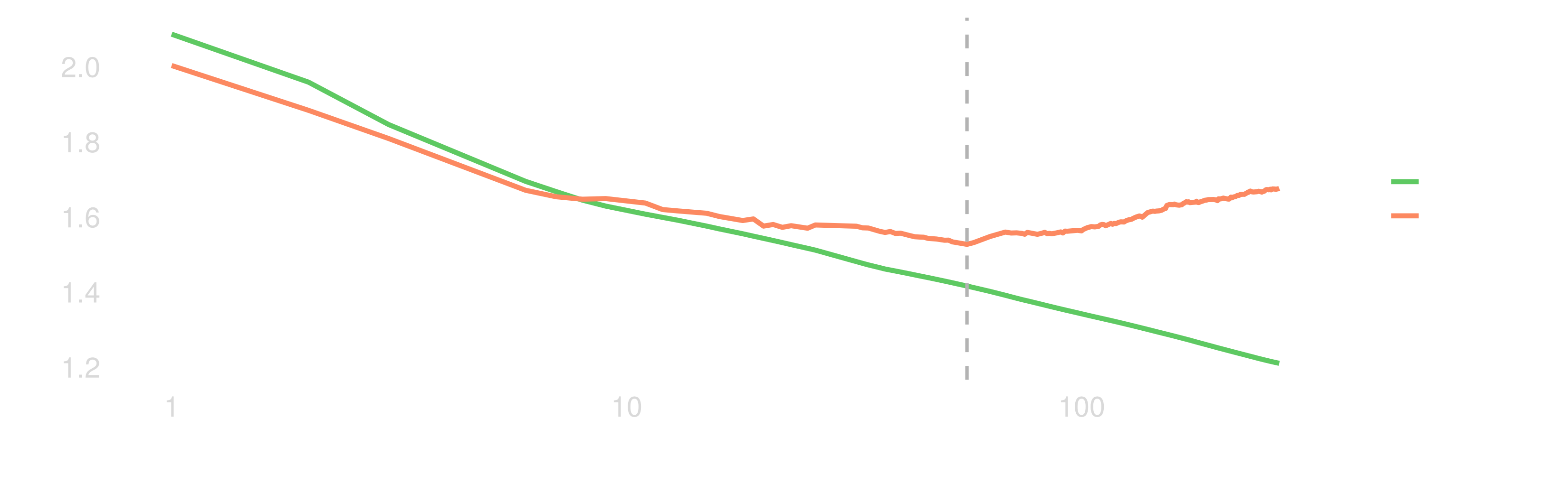
A tree on all nine inputs, grown to 272 leaves, pruned back along its sequence. Training error falls with every leaf; tuning error is lowest at 56 leaves
Trees and missing inputs
The films’ budget is missing for 87%: a film with no budget cannot answer “budget < c?”
Missingness as information: a split also chooses which side the films with no budget go to, like its cutoff, to lower the RSS (xgboost’s default direction); or a budget missing indicator that the tree can split on
Missingness as a nuisance: rpart’s surrogate splits, backup questions on other inputs that send the training films the same way; a film missing the split’s input follows the best backup it can answer
Informative here: budgets were recorded mostly for widely rated films (median 1,238 votes, against 71). Potentially useful for prediction
A downside of trees: variance
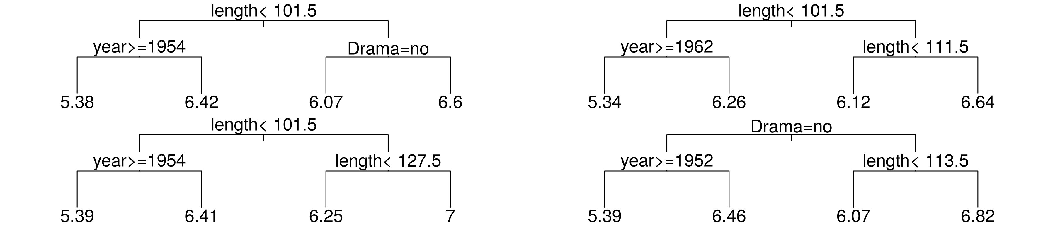
Depth 2, each on a random half of the training films. Star Wars: Episode I - The Phantom Menace (rated 6.4): predicted 6.07, 6.64, 7.00, 5.39
Same method, random halves of the same films, four different models. What should we do?
Part 4: three model improvement strategies
Sacrifice simplicity/interpretability for prediction accuracy
Bagging*: bootstrap aggregating
Resample training data, average resulting models
Random forest
Randomly drop predictors at each split
Boosting*
Successively add simple models to improve the aggregate
* Can be used with other models too, not just trees
Bagging: bootstrap aggregating
Problem: a single tree model can have high variance (like many non-smooth or non-regularized models)
Bootstrap: for each \(b = 1, \ldots, B\) resamples (with replacement) of the training data, fit \(\hat f^b\) on bootstrap sample \(b\)
Aggregate: combine the \(B\) models, using majority vote for classification or mean for regression
Average \(B\) trees’ predictions at one input \(x\) (variance over the draw of the training data, and of the resampling)
What is the variance of their average if the \(B\) trees are
copies of the same tree, with variance \(\tau^2\)?
independent, each with variance \(\tau^2\)?
each with variance \(\tau^2\), every pair with correlation \(\rho\)?
Recall: variance of a sum
For random variables \(V_1, \ldots, V_n\) and constants \(a_1, \ldots, a_n\), every variance plus every covariance: \[
\mathrm{Var}\Big(\sum_{i=1}^n a_i V_i\Big) = \sum_{i=1}^n a_i^2\, \mathrm{Var}(V_i) + \underbrace{\sum_{i=1}^n \sum_{j \neq i} a_i a_j\, \mathrm{Cov}(V_i, V_j)}_{n(n-1) \text{ terms; } \binom{n}{2} \text{ distinct}}
\]
Correlated-average variance
With \(n = B\) and every \(a_i = 1\): \(B\) terms \(\tau^2\) and \(B(B - 1)\) terms \(\rho\tau^2\), \(\;\mathrm{Var}\big(\sum_{b} V_b\big) = B\tau^2 + B(B - 1)\rho\tau^2\)
Correlated-average variance.\(V_1, \ldots, V_B\), each with variance \(\tau^2\), every pair with correlation \(\rho\): \[
\mathrm{Var}\Big(\frac1B \sum_{b=1}^B V_b\Big) = \rho\,\tau^2 + (1 - \rho)\,\frac{\tau^2}{B}
\]
Proof: divide by \(B^2\) and regroup, \(\frac{\tau^2}{B} + \frac{B - 1}{B}\rho\tau^2 = \rho\tau^2 + (1 - \rho)\frac{\tau^2}{B}\). Bagging shrinks the second term; \(\rho\tau^2\) stays, since bootstrap trees grown from one sample are alike
Random forest: dropping predictors
Suppose \(B\) is large, say 300. Which term of the correlated-average variance is left, and how could we make it smaller?
Problem: aggregation does not increase information if the aggregates are highly correlated, e.g. averaging 1000 trees but each one uses the same small set of predictor variables
Drop predictors randomly, at every split
e.g. each split chooses among a random \(\sqrt{p}\) of the \(p\) predictors
Aggregate models which are now (typically) less correlated, achieving greater variance reduction
Out-of-bag predictions
Each bootstrap sample contains some subset of the training data
Roughly \(1/e \approx 0.37\) portion of the training samples will be left out of each bootstrap sample
Can use these to estimate test error (e.g. instead of \(K\)-fold cross-validation)
Software implementations may do this automatically
A forest on the films, 300 trees
MSE
training films, every tree
1.19
training films, out-of-bag trees only
1.50
tuning films
1.49
tuning films, predicting the training mean
2.00
Adding trees
A forest grows its trees separately and averages them. Now grow them one after another and add them up: after \(b\) trees the fit is \(\hat f^{(b)}\), the sum so far
We may add one small tree to \(\hat f^{(b)}\). What should it predict?
The residual from the existing fit: \(y - \hat f^{(b)}(x)\)
Boosting: iterated fitting on residuals
Idea: train models sequentially, decreasing residuals by a small amount each time. Each model contributes something different
Can use “weak learners” (e.g. trees with one split, “stumps”) to grow an ensemble model gradually fitting closer to the training data
Relationship with gradient descent
Gradient descent: small step in direction of negative gradient
Boosting: small step in direction of weak learner approximating the negative gradient
Instead of taking an unrestricted gradient step, we reduce the loss by taking a small step in the direction of a weak learner: a simple, low-cost model
The training loss depends on a model only through its \(n\) fitted values \(\mathbf f = (f_1, \ldots, f_n)\), \(f_i = f(x_i)\): a function of \(n\) numbers \[
L(\mathbf f) = \sum_{i=1}^n \tfrac12 (y_i - f_i)^2, \qquad -\frac{\partial L}{\partial f_i} = y_i - f_i
\] The negative gradient is the residual vector
A gradient step, \(\mathbf f^{(b)} = \mathbf f^{(b-1)} + \gamma\,(\mathbf y - \mathbf f^{(b-1)})\), changes only those \(n\) values. Boosting trees fits a small tree approximating the negative gradient (the residuals) and steps along it, with learning rate\(\gamma\): \[
\hat f^{(0)} = \bar y, \qquad \hat f^{(b)} = \hat f^{(b-1)} + \gamma\, \hat t_b, \qquad \hat t_b \text{ a small tree fitted to } y_i - \hat f^{(b-1)}(x_i)
\]
Boosting in practice
More tuning parameters
Number of trees/steps \(B\), complexity of each tree/model \(d\), regularization/learning rate \(\gamma\). Warning: can now overfit with large \(B\) (unlike bagging/r.f.)
Software may choose them automatically. No guarantee it’s reasonable!
Bagging and boosting
Bagging and forests start with large trees, which have high variance individually, and average them to lower the variance. Boosting starts with weak learners like tree stumps, which have high bias individually, and fits iteratively on residuals to lower the bias
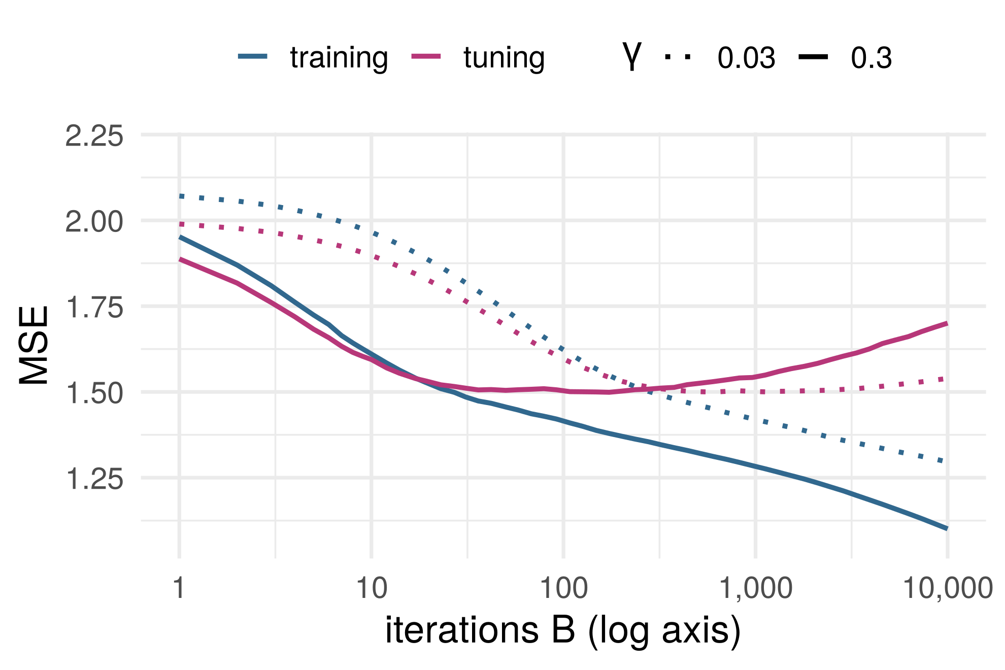
Iterations and learning rate
Iterations \(B\). Training error keeps falling; tuning error turns. Stopping there is early stopping, as for gradient descent
Learning rate \(\gamma\). Smaller steps
Depth. How many inputs one tree can combine (next)
Tree depth and interactions
Can a tree with one split fit \(f(x_1, x_2) = x_1 x_2\) well? Hint: assume the inputs are independent, both \(\mathrm{Unif}[-1, 1]\)
How many splits would we want for \(f(x_1, \ldots, x_p) = x_1 \cdots x_p\)?
A stump asks one question, so a sum of stumps is a sum of one-input functions: an additive model. Depth \(d\): interactions of up to \(d\) inputs
A boosted model is additive in trees, not in the predictors
We’re in dangerous territory
Less interpretable methods/models
Many tuning parameters
Increasingly sophisticated software with many defaults and/or automatically optimized tuning parameters
It is a profoundly erroneous truism, repeated by all copy-books and by eminent people when they are making speeches, that we should cultivate the habit of thinking of what we are doing. The precise opposite is the case. Civilization advances by extending the number of important operations which we can perform without thinking about them.
Conclusion
Additive models
One curve per input, each fitted to what the others leave: partialling out, one input at a time
Additivity vs interactions
A plot of one input at a time works most naturally for additive models, and can be importantly wrong when the truth has interactions
Trees and ensembles
Greedy questions, pruned by validation. Bagging and forests average trees to lower variance; boosting adds small trees, gradient descent on the fitted values
References
Box, G. E. P. (1976). Science and statistics. Journal of the American Statistical Association 71(356), 791–799. doi:10.1080/01621459.1976.10480949. The quotation is in section 2.4.
Box, G. E. P. and Draper, N. R. (1987). Empirical Model-Building and Response Surfaces. New York: Wiley.
Breiman, L., Friedman, J. H., Olshen, R. A. and Stone, C. J. (1984). Classification and Regression Trees. Belmont, CA: Wadsworth.
Chen, T. and Guestrin, C. (2016). XGBoost: a scalable tree boosting system. Proceedings of the 22nd ACM SIGKDD International Conference on Knowledge Discovery and Data Mining, 785–794. doi:10.1145/2939672.2939785
Josse, J., Chen, J. M., Prost, N., Varoquaux, G. and Scornet, E. (2024). On the consistency of supervised learning with missing values. Statistical Papers 65(9), 5447–5479. doi:10.1007/s00362-024-01550-4
Louisiana v. Callais, 608 U.S. 85 (2026), No. 24-109, decided 29 April 2026. Opinion (preliminary print). The quotation is in the syllabus, at 88.
Morris, G. E. (2026). The simple statistical error Republican Supreme Court justices used to gut the VRA. Strength In Numbers, 8 May 2026. Link
Twala, B. E. T. H., Jones, M. C. and Hand, D. J. (2008). Good methods for coping with missing data in decision trees. Pattern Recognition Letters 29(7), 950–956. doi:10.1016/j.patrec.2008.01.010
Whitehead, A. N. (1911). An Introduction to Mathematics. London: Williams and Norgate. Project Gutenberg. The quotation is in chapter 5, “The Symbolism of Mathematics”.