Materials
| Link | Type | Description |
|---|---|---|
| html pdf | Slides | Course introduction |
| html pdf | Slides | Preview of machine learning concepts |
| html | Notebook | gapminder example |
| html | Notebook | candy example |
| html | Notebook | Previous (outdated) seminar |
Updated notebooks will be available on GitHub.
Preparation
Required reading
- ISLR Chapter 1: Introduction. Should be a quick read. Don’t skip the section on Notation and Simple Matrix Algebra.
- ISLR Chapter 2: Statistical Learning.
If you finish these quickly you may want to start Chapter 3, because it’s a long one.
Supplemental reading
Installing R and
RStudio
First install R and then install RStudio (this second step is highly recommended but not required, if you prefer another IDE and you’re sure you know what you’re doing). Finally, open RStudio and install the tidyverse set of packages by running the command
install.packages("tidyverse")Note: If you use a Mac or Linux-based computer you may want to install these using a package manager instead of downloading them from the websites linked above. Personally, on a Mac computer I use Homebrew (the link has instructions for how to install it) to install R and RStudio.
What is machine learning?
We begin with some key conceptual themes in machine learning. The subject mainly focuses on algorithms for finding potentially useful structure in data.
Supervised machine learning
This refers to the special case where one variable in the dataset is specified as an “outcome”–usually represented as \(y\)–the other variables are considered inputs or “predictors”–written as \(x\)–and the algorithm attempts to “fit” a functional relationship between these using the dataset. A key idea in applied mathematics is that there may be some “true” function \(f\) that describes the relationship between \(x\) and \(y\), so that measured data will satisfy
\[ y = f(x) + \epsilon \] where \(\epsilon\) is a (hopefully small) “error” term. In the physical sciences, for example, this function could describe a “law” such as the laws of mechanics or elecromagnetism, etc. In machine learning we usually don’t know the function, or even have good a priori reasons to believe there is a useful functional relationship. Instead we hope that a (powerful enough) algorithm can “learn” a function \(\hat f\) by approximating the examples in a (large enough) dataset:
\[ \hat f(x_i) \approx y_i, \quad \text{ for } \quad i = 1, \ldots, n \] We might only care about the prediction accuracy of this learned function, or we might also want to interpret it based on the assumption that it is close to the “true” function: \[ \hat f(x) \approx f(x) \] Technological advances in computing enable us to use more sophisticated algorithms and achieve better accuracy. This often creates tension between the two goals above, since new “state of the art” (SOTA) algorithms that have the highest prediction accuracy are usually very complicated and hence difficult to interpret. Later in the course we will learn about some algorithmic tools to help us interpret other algorithms.
Model complexity
The distinguishing feature of machine learning as compared to statistics, for example, is that it is mainly concerned with the accuracy of the fitted relationship. In statistics we usually want some kind of inference for our fitted models, for example confidence/prediction intervals, hypothesis tests, and diagnostic plots. Machine learning drops this requirement allowing us to more kinds of models, including ones where we do not know how to compute valid inferences or provide any simple interpretations. To move in the direction of machine learning, then, we can imagine starting at statistics and taking a step in the direction of greater model complexity.
Two simple examples illustrate different strategies for building more complex models:
- increasing complexity of the function class, for example by using (more highly) non-linear functions and/or allowing functions to fit flexibly/locally to different subsets of the data
- increasing the dimension of predictors (while otherwise keeping the function class fixed)
Model complexity relates to the bias-variance trade-off: more complexity typically results in lower bias and higher variance.
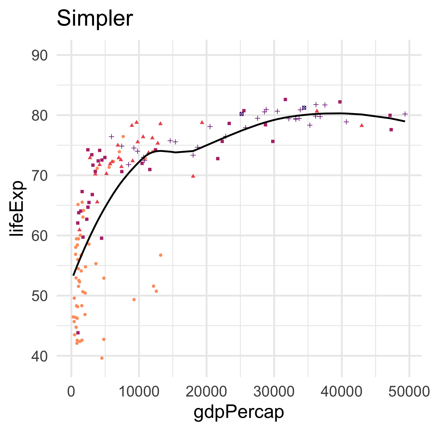
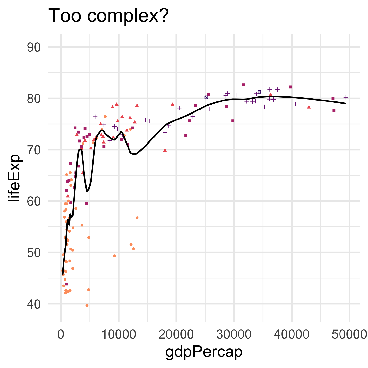
Increasing complexity usually results in a lower mean-squared error if the MSE is calculated on the same dataset that was used to fit the model. But if the MSE is calculated on a different dataset this is no longer true, and more complexity may result in a larger MSE on the other dataset.
Why should we evaluate model fit (like MSE) on a different dataset than the one used to fit the model? First, if we evaluate it on the same dataset instead, then such an evaluation will always prefer greater complexity until the model “saturates” the data. In this case there was nothing gained from using a model–we have only created a map as large as the entire territory. Second, if our purpose in using a model is to describe some stable aspect of the world, if we think the “true” \(f\) is something like a “law of nature,” then we would hope that such a model would not immediately fail if the time or context of the data collection is slightly different.
Since these concepts are so central to machine learning we will return to them several times through the term and understand them through more examples and some mathematical derivations.