Week 3 seminar

Author

Joshua Loftus

Note

This is the student version of the notebook. The code you write goes where a line says # ... or has a ____. A code chunk with a blank starts with #| eval: false, so the file renders as it stands; delete that line once you have filled the blank. Working through the chunks one at a time in RStudio (Ctrl/Cmd+Enter) is unaffected. Answers are revealed in the seminar.

library(tidyverse)       # should've already install.packages("tidyverse")
library(palmerpenguins)  # might need to install.packages("palmerpenguins")
library(broom)           # might need to install.packages("broom")
library(yardstick)       # might need to install.packages("yardstick")
theme_set(theme_minimal())

Before the seminar

The lecture proved one result, the adjustment theorem, which you prove again with the slides closed (exercise 3). It stated the optimal threshold theorem and no free lunch and left proofs to you (exercises 1 and 4), and it stated the confounding gap without deriving it (exercise 2). Do all four on paper before the seminar; the seminar’s problems are variations on exercises 1 to 3. You may use, without proof, two facts from ST102: the tower property, \(\mathbb E[W] = \mathbb E\big[\mathbb E[W \mid X]\big]\), and that if \(V\) is independent of \(X\), then \(\mathbb E[k(X, V) \mid X = x] = \mathbb E[k(x, V)]\) for any function \(k\) (freeze \(X\) at \(x\); the distribution of \(V\) does not move).

Hints

Each exercise has hints, collapsed below it. Do not open a hint unless you have been stuck for at least a few minutes, and open them in order. Exercise 3’s proof is on the lecture slides. Solutions to exercises 1, 2 and 4 are shown in the seminar if you ask.

Exercise 1 (optimal threshold theorem). Let \(p(x) = P(Y = 1 \mid X = x)\). A false positive (predict \(1\), truth \(0\)) costs \(c_{FP} \ge 0\), a false negative (predict \(0\), truth \(1\)) costs \(c_{FN} \ge 0\), not both are \(0\), and a correct prediction costs nothing. A rule \(\delta\) assigns a prediction \(\delta(x) \in \{0, 1\}\) to every \(x\).

At a fixed \(x\), write the expected cost of predicting \(1\) and the expected cost of predicting \(0\).
Show that predicting \(1\) has the smaller expected cost exactly when \(p(x) > c^\star = c_{FP}/(c_{FP} + c_{FN})\). What happens at \(p(x) = c^\star\)?
Let \(\delta^\star\) be the rule from (b). Show that \(\mathbb E\big[\text{cost}(\delta^\star(X), Y)\big] \le \mathbb E\big[\text{cost}(\delta(X), Y)\big]\) for every rule \(\delta\).
With equal costs, what is \(c^\star\), and what is the probability of a wrong label at \(x\) under \(\delta^\star\)?

Hint 1

Given \(X = x\), \(Y\) is \(1\) with probability \(p(x)\). If you predict \(1\), when is that a mistake, and what does the mistake cost?

Hint 2

Compare the two expected costs and solve the inequality for \(p(x)\). “Not both \(0\)” is what lets you divide.

Hint 3

Condition on \(X\) first (the tower property), as in week 2’s exercise 1. What do you know about the inner expectation, at every \(x\)?

Exercise 2 (confounding gap). The lecture’s DAG made linear. \(Z\), \(\varepsilon_T\) and \(\varepsilon_Y\) are independent, \(\varepsilon_T\) and \(\varepsilon_Y\) have mean \(0\), \(\mathrm{Var}(T) > 0\), and \[ T = \alpha Z + \varepsilon_T, \qquad Y = \tau T + \gamma Z + \varepsilon_Y. \]

Under \(do(T = t)\), which variables keep their values? Show that \(\mathbb E[Y \mid do(T = t)] = \tau t + \gamma\, \mathbb E Z\), so that moving \(t\) from \(0\) to \(1\) changes the mean of \(Y\) by \(\tau\).
As observed, show that \(\mathbb E[Y \mid T = t] = \tau t + \gamma\, \mathbb E[Z \mid T = t]\), and hence \[ \mathbb E[Y \mid T = 1] - \mathbb E[Y \mid T = 0] = \tau + \gamma\,\big(\mathbb E[Z \mid T = 1] - \mathbb E[Z \mid T = 0]\big). \] Where did you use independence?
Show that the population slope of the least-squares line of \(Y\) on \(T\) alone, \(\mathrm{Cov}(T, Y)/\mathrm{Var}(T)\), is \(\tau + \gamma\,\delta\) with \(\delta = \mathrm{Cov}(Z, T)/\mathrm{Var}(T)\). Which quantity in week 2’s omitted-variable bias plays the role of \(\delta\)?
When is the gap zero?

Hint 1

Delete \(T\)’s equation and set \(T = t\). Is \(Z\) upstream or downstream of \(T\)?

Hint 2

Take \(\mathbb E[\,\cdot \mid T = t]\) of \(Y\)’s equation term by term. \(T\) is a function of \(Z\) and \(\varepsilon_T\); what does that say about \(\varepsilon_Y\) and \(T\)?

Hint 3

Expand \(\mathrm{Cov}(T, Y)\) using \(Y\)’s equation. \(\mathrm{Cov}(T, \varepsilon_Y) = 0\) for the reason you found in (b).

Exercise 3 (adjustment theorem). The lecture proved this one. Close the slides and prove it again. Structural model: \(Z\), \(\varepsilon_T\) and \(\varepsilon_Y\) independent, \(T = h(Z, \varepsilon_T)\), \(Y = g(T, Z, \varepsilon_Y)\); under \(do(T = t)\) the equation for \(T\) is deleted, \(T\) is set to \(t\), and everything else keeps its equation and its noise. Show that, wherever \(P(T = t \mid Z) > 0\), \[ \mathbb E[Y \mid do(T = t)] = \mathbb E_Z\Big[\,\mathbb E[Y \mid T = t, Z]\,\Big], \] and say where each assumption is used: the independence of the noises, \(Z\) not being a consequence of \(T\), and \(P(T = t \mid Z) > 0\).

Hint 1

Start from the intervened world. What is \(Y\) under \(do(T = t)\), and which variables keep their values? Give the average over the noise with \(Z\) frozen a name: \(m_t(z) = \mathbb E\big[g(t, z, \varepsilon_Y)\big]\).

Hint 2

Use the second ST102 fact, with \(V = \varepsilon_Y\) and \(Z\) in the role of \(X\), to show \(\mathbb E[Y \mid do(T = t)] = \mathbb E_Z\big[m_t(Z)\big]\).

Hint 3

Now the observed world: on \(\{T = t, Z = z\}\), \(Y = g(t, z, \varepsilon_Y)\). Why is \(\varepsilon_Y\) independent of \((T, Z)\), and what does that give for \(\mathbb E[Y \mid T = t, Z = z]\)?

Hint 4

Why is the distribution of \(Z\) the same in the observed and the intervened worlds?

Exercise 4 (no free lunch on a finite domain). A finite set \(\mathcal X\) has \(N\) points. A labeling is a function \(f: \mathcal X \to \{0, 1\}\). A method sees the labels on a fixed training set \(S \subset \mathcal X\) of \(m < N\) points and returns a classifier \(\hat h\), which may be any function of those \(m\) labels. Its error on the points it has not seen is \[ \mathrm{err}(\hat h, f) = \frac{1}{N - m} \sum_{x \notin S} \mathbb 1\big[\hat h(x) \ne f(x)\big]. \]

Draw \(f\) uniformly at random from all \(2^N\) labelings. Show that \(\mathbb E\big[\mathrm{err}(\hat h, f)\big] = \tfrac12\) for every method.
Two methods, \(A\) and \(B\). Suppose \(A\)’s error on the unseen points is smaller than \(B\)’s for some labeling. Show that \(B\)’s is smaller than \(A\)’s for another labeling.
What would have to be true of the world for some method to do better than \(\tfrac12\) on average?

Hint 1

Uniform over all \(2^N\) labelings means that the \(N\) labels \(f(x)\) are independent fair coin flips.

Hint 2

Fix \(x \notin S\). \(\hat h(x)\) depends only on the labels on \(S\), and \(f(x)\) is independent of them. Condition on the labels on \(S\): what is \(P\big(\hat h(x) \ne f(x)\big)\)?

Hint 3

Average \(\mathrm{err}(\hat h_A, f) - \mathrm{err}(\hat h_B, f)\) over all \(2^N\) labelings.

Problems

Problem 1 (costs 5 and 1). A conservation survey classifies penguins from a photograph. Labeling a Chinstrap as an Adelie (a miss) wastes a return visit, cost 5; labeling an Adelie as a Chinstrap (a false alarm) wastes a phone call, cost 1. Write \(p(x) = P(\text{Chinstrap} \mid x)\).

Find the threshold on \(p(x)\) above which predicting Chinstrap has the smaller expected cost. What happens at the threshold itself?
A fitted model gives \(\hat p = 0.25\) for one bird. What does the rule predict, and what would have to be true of \(\hat p\) for that prediction to be the best one at that \(x\)?
The survey hands the same \(\hat p\) to two field teams. For team A a miss costs 5 and a false alarm 1; for team B both cost 1. For which values of \(\hat p\) do the two teams make different calls?
Say in one sentence what the survey decided when it chose 5 and 1.

Problem 2 (the lecture’s DAG, with numbers). Let \(Z\) have mean \(0\) and variance \(1\); let \(T = Z + \varepsilon_T\) and \(Y = T + 2Z + \varepsilon_Y\), where \(\varepsilon_T\) and \(\varepsilon_Y\) have mean \(0\) and variance \(1\), and \(Z\), \(\varepsilon_T\), \(\varepsilon_Y\) are independent.

What is the effect on \(\mathbb E[Y]\) of raising \(t\) by one under \(do(T = t)\)?
Compute \(\mathrm{Var}(T)\), \(\mathrm{Cov}(T, Y)\) and the population slope of the regression of \(Y\) on \(T\) alone. Write it as “effect plus gap” and identify the gap.
Compute \(\mathbb E[Y \mid T = t, Z = z]\), average it over \(Z\), and check that you recover (a). Where did you use that the noises are independent?
A world where the causation runs the other way: \(Y = \varepsilon_Y\) with variance \(4\), and \(T = 0.4\,Y + \varepsilon_T\), with \(\varepsilon_T\) of variance \(0.16\), independent of \(Y\). Find the population slope of \(Y\) on \(T\) and the effect of raising \(t\) by one.

Optional, can be done at home

Problem 3 (what no free lunch says). Which of these claims does exercise 4 support? (a) “Nearest neighbors is a better method than linear regression.” (b) “On the gapminder data, nearest neighbors beat the line.” (c) “A method that makes no assumptions would beat all the others.”

Hint 1

For each claim: is it about one distribution, every distribution, or the average over all labelings?

Problem 4 (a model that predicts well). A hospital fits a model that predicts which patients will be readmitted within 30 days, and it predicts well on held-out patients. Management proposes to reduce readmissions by acting on the model’s strongest predictor. Draw the DAGs of three worlds consistent with that held-out score, say in which of them the plan works, and say what the score told you about which world you are in.

Hint 1

The lecture’s three worlds: the predictor causes readmission, a common cause drives both, or readmission risk drives the predictor.

Coding

1. Penguins: a probability and a threshold

Adelie against Chinstrap, from the bill. Keep the two species and the birds with complete measurements.

pg <- palmerpenguins::penguins |>   # modeldata also has a penguins; be explicit
  filter(species != "Gentoo") |>
  drop_na(bill_length_mm, bill_depth_mm, flipper_length_mm) |>
  mutate(chinstrap = as.numeric(species == "Chinstrap"))
ggplot(pg, aes(bill_length_mm, bill_depth_mm, colour = species)) +
  geom_point() +
  scale_colour_viridis_d(end = 0.7)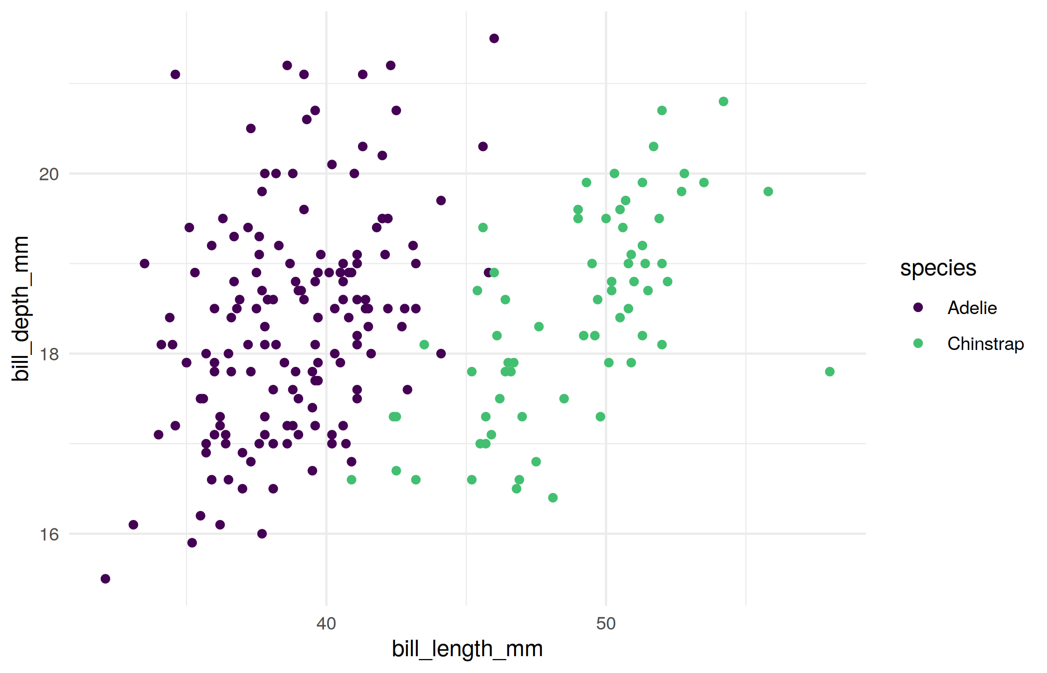

Step 1. How many birds, and what proportion are Chinstraps? What accuracy would a classifier that always predicts the more common species achieve?

# nrow(pg); mean(pg$____)
# max(____, 1 - ____)
# ...

Step 2. Fit the logistic regression of chinstrap on the two bill measurements with glm(..., family = binomial). Look at tidy(), then at tidy(..., exponentiate = TRUE).

# fit_bill <- glm(____ ~ ____ + ____, family = binomial, data = pg)
# tidy(fit_bill)
# tidy(fit_bill, exponentiate = TRUE)
# ...

Checkpoint (run it; if it stops, fix step 2 before going on):

stopifnot(inherits(fit_bill, "glm"), length(coef(fit_bill)) == 3,
          all(fitted(fit_bill) >= 0 & fitted(fit_bill) <= 1))

You may have seen a warning that fitted probabilities are numerically 0 or 1: the two species are nearly separable on these two measurements (step 3 counts the errors). This is the lecture’s “Challenges” slide in real life; next week says what it does to the fitting.

Question 1. Read the exponentiated coefficient on bill_length_mm. What happens to the odds of Chinstrap when bill length increases by one millimeter and bill depth is held fixed? Is that the change in the probability? Is it what would happen to a bird whose bill grew by a millimeter?

Step 3. The confusion matrix at threshold \(\tfrac12\), with table(). From it, compute the accuracy, the true positive rate and the false positive rate.

# p_hat <- fitted(fit_bill)
# tab <- table(truth = pg$chinstrap, predicted = as.numeric(p_hat > ____))
# tab
# accuracy <- (tab[1, 1] + tab[2, 2]) / sum(tab)
# tpr <- ____ ; fpr <- ____
# ...

Checkpoint:

stopifnot(sum(tab) == nrow(pg), tpr >= 0, tpr <= 1, fpr >= 0, fpr <= 1)

Step 4. The bill model is nearly perfect, so it cannot show the trade-off. Fit a weaker model on flipper_length_mm alone, then compute the ROC curve yourself: for thresholds from 0 to 1, the true positive rate and the false positive rate. Plot one against the other. The loop is set up; you write the two rates.

fit_flipper <- glm(chinstrap ~ flipper_length_mm, family = binomial, data = pg)
pg <- pg |> mutate(p_flipper = fitted(fit_flipper))
thresholds <- seq(0, 1, by = 0.01)
roc_by_hand <- map_dfr(thresholds, function(t) {
  yhat <- as.numeric(pg$p_flipper > t)
  # tibble(t = t,
  #        tpr = sum(yhat == 1 & pg$chinstrap == 1) / sum(____),
  #        fpr = sum(____) / sum(____))
  # ...
})
# ggplot(roc_by_hand, aes(____, ____)) + geom_path() + coord_equal()
# ...

Checkpoint:

stopifnot(nrow(roc_by_hand) == length(thresholds),
          all(roc_by_hand$tpr >= 0 & roc_by_hand$tpr <= 1),
          roc_by_hand$tpr[1] == 1, roc_by_hand$fpr[1] == 1)

Question 2. The area under your curve equals the probability that a randomly chosen Chinstrap gets a higher fitted probability than a randomly chosen Adelie, with a tie counting half. Why does accumulating one point per threshold produce that probability? Why are ties certain to occur with this model?

Step 5. Costs. A miss costs 5, a false alarm 1. For each threshold compute the cost per bird on the 219 birds, \(5 \cdot (\text{misses}/n) + 1 \cdot (\text{false alarms}/n)\), find the threshold that minimizes it, and compare with problem 1’s threshold.

# costs <- map_dfr(thresholds, function(t) {
#   yhat <- as.numeric(pg$p_flipper > t)
#   tibble(t = t, cost = (5 * sum(____) + 1 * sum(____)) / nrow(pg))
# })
# ggplot(costs, aes(t, cost)) + geom_line()
# costs |> slice_min(cost, n = 3)
# ...

Checkpoint:

stopifnot(nrow(costs) == length(thresholds), all(costs$cost >= 0))

Question 3. The cost-minimizing threshold is well below \(\tfrac12\), and the classifier now raises many false alarms. Who decided that, and in what sense is this classifier “better” than the one at \(\tfrac12\)? Is the number you found the population optimum?

Optional, can be done at home: the same with `yardstick`

yardstick computes the confusion matrix, the ROC curve and the AUC. It wants factors, and the event_level = "second" argument tells it that 1 is the class of interest.

# pg_y <- pg |> mutate(truth = factor(chinstrap),
#                      predicted = factor(as.numeric(p_hat > 0.5), levels = c(0, 1)))
# conf_mat(pg_y, truth = truth, estimate = predicted)
# roc_curve(pg_y, truth, p_flipper, event_level = "second") |> autoplot()
# roc_auc(pg_y, truth, ____, event_level = "second")
# ...

2. Four worlds, and the adjustment theorem in code

Four simulated worlds in which \(Y\) is regressed on \(X\). In the lecture the target variable was called \(T\); here it is X, because T is TRUE in R. The function draws the noise once and keeps it, so that an intervention can be computed for the same units. World D is the lecture’s DAG with the confounder \(Z\) observed: \(Z \to X\), \(Z \to Y\), \(X \to Y\).

simulate_world <- function(world, n = 500) {
  e_u <- rnorm(n)
  e_x <- rnorm(n)
  e_y <- rnorm(n)
  if (world == "A") {           # X causes Y
    X <- e_x
    Y <- 2 * X + e_y
    Z <- NA
  } else if (world == "B") {    # U causes both; U is not observed
    U <- e_u
    X <- U + 0.5 * e_x
    Y <- 2.5 * U + e_y
    Z <- NA
  } else if (world == "C") {    # Y causes X
    Y <- 2 * e_y
    X <- 0.4 * Y + 0.4 * e_x
    Z <- NA
  } else {                      # D: Z causes both, and X causes Y; Z is observed
    Z <- e_u
    X <- 5 - 2 * Z + e_x
    Y <- 4 + 2 * Z - 3 * X + e_y
  }
  tibble(world = world, X = X, Y = Y, Z = Z, e_u = e_u, e_x = e_x, e_y = e_y)
}
worlds <- bind_rows(simulate_world("A"), simulate_world("B"), simulate_world("C"), simulate_world("D"))

Step 1. In each world, fit lm(Y ~ X) and report the slope.

# worlds |>
#   group_by(world) |>
#   summarise(slope = coef(lm(____))[2])
# ...

Question 4. Before you intervene: for each world, write down what you expect to happen to \(Y\) when \(X\) is set to \(X + 1\) for every unit with the same noise, and the average change. Use each world’s equations, and exercise 2 for world D.

Step 2. Now intervene: set \(X\) to \(X + 1\) for every unit and recompute \(Y\) with the same noise, following each world’s equations. Write the four Y_do lines and compute the average change in \(Y\) in each world.

intervene <- function(d) {
  d |> mutate(
    X_do = X + 1,
    # Y_do = case_when(
    #   world == "A" ~ ____,
    #   world == "B" ~ ____,
    #   world == "C" ~ ____,
    #   world == "D" ~ ____
    # )
    # ...
  )
}
worlds_do <- intervene(worlds)
worlds_do |>
  group_by(world) |>
  summarise(slope = coef(lm(Y ~ X))[2],
            effect_of_intervention = mean(Y_do - Y))

Checkpoint:

stopifnot(all(c("X_do", "Y_do") %in% names(worlds_do)),
          abs(mean(worlds_do$Y_do[worlds_do$world == "C"] - worlds_do$Y[worlds_do$world == "C"])) < 1e-8)

The average change is the average treatment effect of the intervention, \(\mathbb E[Y \mid do(X = x + 1)] - \mathbb E[Y \mid do(X = x)]\), computed on these units: exactly \(2\), \(0\), \(0\) and \(-3\), because the noise was reused.

Step 3. World D, the adjustment theorem in code. Regress Y on X and Z and read off the coefficient on X. Then do what the theorem says: fit \(\hat m(x, z)\) for \(\mathbb E[Y \mid X = x, Z = z]\) (the same regression), evaluate it at every unit’s \(Z\) with \(X\) set to \(X + 1\) and to \(X\), and average the difference.

d <- worlds |> filter(world == "D")
# fit_d <- lm(Y ~ ____ + ____, data = d)
# tidy(fit_d)
# mean(predict(fit_d, newdata = mutate(d, X = ____))) - mean(predict(fit_d, newdata = d))
# ...

Question 5. The coefficient on X and the averaged difference are the same number, and both are near \(-3\). Which result says the coefficient estimates the effect, which says the averaged difference does, and what about world D made both work? What would go wrong in world B, where the confounder e_u is in the table but would not be observed in practice?

Question 6. Redraw the noise in intervene() (replace e_y by rnorm(n())) and look at Y_do - Y unit by unit in world A. What changes, and what does not? Which version is the counterfactual for a unit, and which is a new draw from the intervened world?

Optional, can be done at home: another dataset

Attrition (modeldata::attrition; fictional, made up by IBM data scientists, used only as an exercise): whether an employee leaves, with a threshold-and-costs story (a missed leaver costs a replacement, a false alarm costs a conversation). Leavers are 16 percent, so the accuracy-against-cost point is sharper: at threshold \(\tfrac12\) almost nobody is predicted to leave.

library(modeldata)
data(attrition)
att <- attrition |> mutate(left = as.numeric(Attrition == "Yes"))
fit_att <- glm(left ~ OverTime + MonthlyIncome + Age + JobSatisfaction, family = binomial, data = att)
# then steps 3, 4 and 5 with p = fitted(fit_att), costs 10 (a missed leaver) and 1 (a false alarm)
# ...

Before the seminar

Problems

Optional, can be done at home

Coding

1. Penguins: a probability and a threshold

Optional, can be done at home: the same with yardstick

2. Four worlds, and the adjustment theorem in code

Optional, can be done at home: another dataset

Optional, can be done at home: the same with `yardstick`